
Chapter 8
Developing and Evaluating Alternatives
C. Robert Kenley
School of Industrial Engineering, Purdue University, West Lafayette, IN, USA
Clifford Whitcomb
Systems Engineering Department, Naval Postgraduate School in Monterey, Monterey, CA, USA
Gregory S. Parnell
Department of Industrial Engineering, University of Arkansas, Fayetteville, AR, USA
Truly successful decision making relies on a balance between deliberate and instinctive thinking.
Malcolm Gladwell, Blink: The Power of Thinking Without Thinking, 2005
8.1 Introduction
As discussed in Chapter 1, value identification requires that we create feasible alternatives. We also need techniques for evaluating alternatives that measure the value of each alternative and identify the alternatives that provide the most potential value, as presented in Chapter 2. This chapter reviews techniques for creating and evaluating alternatives, provides references for the techniques, and provides an assessment of the techniques. When using the methods in this chapter, always keep in mind the decision traps discussed in Section 6.3.
This chapter is organized as follows: Section 8.2 presents an overview of decision-making, creativity, and teams, and Section 8.3 presents techniques for creating alternatives. These sections describe divergent and convergent phases for alternative development, and when techniques are embedded in what is customarily proposed as a complete process for creating and evaluating alternatives, it identifies and describes the embedded alternative development techniques. Section 8.4 assesses the alternative creation techniques with respect to when they are best applied during the life cycle and their contribution to the divergent and convergent phases of alternative development. Section 8.5 presents alternative evaluation techniques, including the techniques embedded in complete processes for alternative development and evaluation. Section 8.6 assesses the alternative evaluation techniques with respect to best practices for making good decisions (Howard & Abbas, 2016) along the dimensions of information, preferences, and logic. The chapter concludes with key terms, exercises, and references.
8.2 Overview of Decision-making, Creativity, and Teams
The section provides an overview of three important areas that are relevant to developing alternatives.
First, decision-making approaches vary according to the decision opportunity. It is important to understand the characteristics of the decision opportunity and approaches that are applicable to the situation before committing to complete a trade study when perhaps another approach may be more appropriate.
Second, research in engineering design has identified the cognitive methods that are the most effective for creating alternatives. The research results are not surprising to those who have experience with approaches that are employed by highly skilled system engineers. We believe it is critically important to create innovative alternatives before taking the deep dive into decision calculus that provides analytic insights into the trade-offs between the alternatives.
Finally, due to multiple stakeholder objectives, uncertainties about competition and adversaries, and the complexity of systems, we need expertise in many areas to perform a quality trade-off analysis – trade studies are a team sport. Research in the psychology of teams has identified personality-based suggestions for improving the performance of individuals in a team environment, the roles that must be balanced when building a team, and the tasks that are more appropriate for individuals versus being completed as a team exercise.
8.2.1 Approaches to Decision-Making
Table 8.1 summarizes three modes of decision-making from Watson & Buede (1987, 123–124) that characterize different approaches to making decisions that are appropriate for different decision opportunities. The “Choosing” mode employs decision analysis methods and is the principal approach used for performing trade-off analyses. The “Allocating” mode captures decision-making approaches that apply optimization techniques that distribute scarce resource(s) among competing projects. This mode is typical for operations research and multidisciplinary design optimization. Also included in the allocating mode is the determination of constraints based on physics (Slepian 1963) and on the laws of probability (Kenley & Coffman, 1998). The “Negotiating” mode captures decision-making approaches that apply game theory and agent-based modeling to understand the dynamics of multiple interacting decision-makers. Negotiating includes mechanism design, which is the design of the rules that provide for a situation that is efficient, effective, and fair for all parties.
Table 8.1 The Modes for Making Decisions
| Mode | Definition | Distinctive Traits of the Decision Opportunity | Common Methods |
| Choosing | Selecting one alternative from a list |
|
|
| Allocating | Distributing scarce resource(s) among competing projects |
|
|
| Negotiating | Defining an agreement with one or more actors |
|
|
8.2.2 Cognitive Methods for Creating Alternatives
The quality of any decision-making, no matter what mode is employed, is dependent on generating a range of decision alternatives that provide multiple means for achieving the objectives of the decision-makers and stakeholders. Jones (1992) indicates that the range and structure of alternatives to be searched at the system level change form based on assumptions made and the willingness of others to adopt the design solutions. The decision alternatives are characterized by variables that parameterize the discrete and continuous choices that are available and by the sequential ordering of the choices, which may include choices to gather additional information about contextual or environmental factors. This additional information may result in an update to the assumptions, and it may increase the willingness of decision-makers to commit to taking action.
Results from research on design methods highlight the importance of two key methods for effectively generating alternatives: visualization and organizing information according to functionality. Cross (2000) states that the ability to design depends on both internal (in the mind's eye) and external (on the whiteboard) visualizations such as drawings and that designers employ these visualizations to structure the design space and generate alternatives. Cross also notes that visualization enables designers to work simultaneously with the overall concept and lower-level details that have a critical influence on the overall design. Ullman (2010) explains that experienced designers use functional groupings as an indexing mechanism to generate information about design options and that the information typically is a graphical representation of the structure of the options rather than the values of specific physical parameters. Fortunately, for trade studies performed within the context of an overall systems engineering approach, visual and functional representations of the problem space and the design space are commonly used, and a trade study team should make every effort to take advantage of the visual and functional modeling artifacts that the system design team has developed.
8.2.3 Key Concepts for Building and Operating Teams
Complex system designs require a large number of designers and systems engineers. These individuals usually work in teams within and across organizational boundaries.
Extensive research (McGrath, 1984) indicates that individuals working separately generate many more ideas than do groups. Two-part group methods such as the nominal group technique that allow for initial generation of concepts by individuals and follow-up in group sessions to enhance concepts were found to be very effective in taking advantage of the concept generation capabilities of individuals. These two-part methods provide the proper balance between generating alternatives and achieving the group buy-in needed to avoid down-selecting alternatives prematurely. In addition, decision-makers who participate in the group sessions should be more willing to commit to recommendations from the decision-making process than if they were left out of the process altogether.
Belbin (2010) describes nine team roles for team members by identifying the role name, the characteristics of individuals in the role, and the key activities the individual performs as shown in Table 8.2.
Table 8.2 Belbin's Nine Roles for Team Members
| Role | Characteristics | Key Activities |
| Plant | Creative, imaginative, unorthodox | Solves difficult problems |
| Resource investigator | Extrovert, enthusiastic, communicative | Explores opportunities. Develops contacts |
| Coordinator | Mature, confident, a good chairperson | Clarifies goals, promotes decision-making, and delegates well |
| Shaper | Challenging, dynamic, thrives on pressure | Has the drive and courage to overcome obstacles |
| Monitor-Evaluator | Sober, strategic, discerning | Sees all options. Judges accurately |
| Team Worker | Cooperative, mild, perceptive, diplomatic | Listens, builds, averts friction, and calms the waters |
| Implementer | Disciplined, reliable, conservative, efficient | Turns ideas into practical actions |
| Completer-Finisher | Painstaking, conscientious, anxious | Searches out errors and omissions. Delivers on time |
| Specialist | Single-minded, self-starting, dedicated | Provides knowledge and skills in rare supply |
Belbin indicates that balancing these roles among team members is crucial to achieving successful outcomes and that these team roles are distinct from the functional roles that team members fulfill in accordance with their formal job descriptions. Belbin provides guidance for building and operating teams to ensure that the team roles effectively balanced.
Ullman (2010) describes five problem-solving dimensions of individuals that are relevant to their performance on teams and provides suggestions for the most effective approaches to contributing to team success along these dimensions:
- Problem-solving style (extroverted vs introverted)
- Information management style (preference to work with facts vs with possibilities)
- Information language (verbal vs visual)
- Deliberation style (objective vs subjective)
- Decision closure style (decisive vs flexible).
Ullman provides suggestions on maximizing the productivity of individuals in a team environment organized along these dimensions that are summarized in Table 8.3.
Table 8.3 Ullman's Suggestions for Increasing Team Performance
| Problem-Solving Dimension | Suggestions for Increasing Team Performance |
| Problem-solving style | Externals need to
Internals need to
|
| Information management style | Fact-oriented members need to
Possibility-oriented team members need to
|
| Information language | Team leaders need to
|
| Deliberation style | Objective team members need to
|
Subjective team members need to
|
|
| Decision closure style | Flexible team members need to
Decisive team members need to
|
8.3 Alternative Development Techniques
Alternative development should be a two-phase process. The first phase is divergent thinking that results in creating many ideas. The second phase is convergent thinking that requires organized, analytic thinking to identify a smaller number of well-crafted, feasible alternatives for the initial evaluation. Once the initial evaluation is complete, the process should be repeated to refine and improve the alternatives (Figure 8.1).
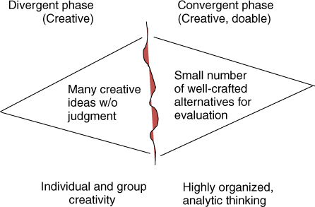
Figure 8.1 Two phases of alternative development (Source: Parnell et al. 2013. Reproduced with permission of John Wiley & Sons)
8.3.1 Structured Creativity Methods
Creativity is a critical aspect for successfully executing the divergent phase when engineering new products and systems. It is “the ability to transcend traditional ideas, rules, patterns, relationships, or the like, and to create meaningful new ideas, forms, methods, interpretations, and so on; originality, progressiveness, or imagination” (Dictionary.com). Structured methods provide useful approaches for an individual or a system development team to think about problems and to create solutions. The concepts for building and operating teams described in Section 8.2.3 should be applied when using structured methods to create an environment that generates many alternative viewpoints and does not yield to pressures toward uniformity, which lead to seeking consensus and eliminating alternatives too early in the process.
Several representative methods are outlined, although many others are available. The methods covered are brainstorming, Reversal, SCAMPER, Six Thinking Hats, Gallery, and Force Field.
- Brainstorming. This method can be either an individual exercise or a group exercise. In groups, the objective of this method is to generate within a given time limit as many ideas as possible for solving a problem. Having ground rules and posting them where all participants can see them is useful to keep everyone aware of the rules before and during the process. All members of the group should participate and, if someone has not participated, someone in the group should ask that person to give an idea. Ideas are recorded with no criticism or evaluation of ideas from the other participants. Encourage participants to augment and enhance others' ideas. Do not let single participants do too much explaining or digressing or giving all the idea inputs. Enthusiastic participation by everyone keeps the process moving. If the process reaches a lull, then try to get new ideas by kick-starting the conversation. When the time limit is reached, or the ideas stop coming, stop the process. Make sure to record the ideas, either on a computer that can be displayed on a video screen or using a white board or flip chart, so that everyone can see them, consider what has been offered, and use them to generate new ideas. Once documented, the ideas can then be used in various ways to see how they might apply to the problem, with constructive feedback and making sure that the process moves to convergence on one or several possible best ways forward.
- Gallery. This method is implemented by having team members write down ideas about the system problem at hand, either on computer or flip chart paper or on sticky notes, which are then placed on a sheet of flip chart paper or poster board – or even individually partitioned parts of a white board. Set a time limit for participants to generate their ideas. Post the resulting posters or flip chart papers on a wall, and have the group of participants walk around the room individually or in informal groups to view the posters as if they were in a gallery. Having participants place their own notes on desired posters will allow everyone to add their comments. The person who created each poster can then present their summary to the group. This method has the advantage of allowing those who do not like to present their ideas in a group setting to get their ideas out in front of everyone through a more private idea generation process. The group gets to review everything and has a chance to comment before the group discussions.
- Reversal. This method has participants take contrary or opposite positions by responding to questions about what you would not like to have happen to your product or system. By taking the opposite position, ways to prevent this outcome may become clear, so you can make sure that the system does not let these things happen. The method has the advantage of allowing participants to state openly some of the ways a system can fail in a noncritical environment so they can be considered, especially during the system conceptualization and design stages.
- SCAMPER. Bob Eberle (1996) created this method that uses a set of techniques that define different ways to approach thinking about a problem. The use of the various techniques forces thinkers to apply methods, including ones that they might not have considered for application to the problem at hand. A key point is to force a response from each perspective and, thus, provide many possibilities to expand thinking. Some responses may end up not being feasible and should be eliminated. For SCAMPER, the seven ways to think about a system problem are as follows:
- Substitute – Remove something from a solution or alternative, and substitute it with something else.
- Combine – Put together two or more system aspects in ways that yield a new solution or possibility.
- Adapt – Change something about the system, so it does something it could not before the change.
- Modify – For the attributes of the system, make changes, even arbitrarily, and study the results or possibilities.
- Put to Other Use – Alter the intention of the system. Challenge assumptions about the system, and suggest new purposes.
- Eliminate – Arbitrarily take out some or all parts of the system or solution to simplify the solution or to use as a basis to find a way to proceed without what was eliminated.
- Reverse – Change the orientation (turn it upside down, invert it, etc.) or direction (go backward, against typical direction, etc.) of the system or components.
- Six Thinking Hats. This method (De Bono, 1985) forces participants to take on different perspectives about a problem based on the hat they wear, substituting that perspective for one that they might have used themselves:
- The White Hat calls for information known or needed based on facts.
- The Yellow Hat symbolizes brightness and optimism and explores the positives and probes for value and benefit.
- The Black Hat uses judgment to articulate why something may not work.
- The Red Hat signifies feelings, hunches, and intuition and calls for expressing emotions and feelings and sharing fears, likes, dislikes, loves, and hates.
- The Green Hat focuses on creativity to generate possibilities, alternatives, and new ideas and allows for expressing new concepts and new perceptions.
- The Blue Hat manages the thinking process and ensures that the overall process guidelines are observed.
- Force Field. This method was developed by Lewin (1943) to consider all the forces that come to play on a system. The process begins with a brief problem statement, and then participants add all the forces that might either help or hinder the process or system from going forward toward a solution. Each idea is categorized as either “help” or “hinder.” Arrows are shaped around each idea, with the direction indicating help or hinder and size indicating the relative magnitude of the force. The overall process outcome is to identify the forces and combination of forces that exist and to then strengthen the helping (positive) ones and to weaken the hindering (negative) ones.
8.3.2 Morphological Box
Morphology has been used in many fields of science, such as anatomy, geology, botany, and biology, to designate research on structural interrelations. Fritz Zwicky generalized and systematized morphological research and applied it to abstract structural interrelations among phenomena, concepts, and ideas for the purpose of discovery, invention, research, and construction of approaches to deal with all situations in life more effectively (Zwicky, 1969, 273). Zwicky's principal tool is the morphological box, chart, or table that is constructed using different dimensions that define a multivariate decision space. A morphological box provides a structure for divergent thinking that generates multiple decision alternatives and for first-order convergent thinking that eliminates unreasonable and unachievable alternatives. There are three variants of the morphological box described in this section: the functional allocation box, the physical architecture definition box, and the strategy table.
8.3.2.1 The Functional Allocation Box
Ullman (2010) describes a technique for designing with function that constructs a morphological box to create the alternatives by defining physical means for accomplishing the system's functions as shown in Figure 8.2. The alternatives are all possible combinations of the means for all of the functions. Assuming that the last three functions listed in Figure 8.2 are constrained to be achieved by the same means, there are ![]() = 640 alternatives that can be created from this morphological box. Of course, not all 640 combinations are reasonable or even physically achievable. For example, if a cantilever is used to transmit the vertical force to the body, then it is reasonable to use it to transmit the horizontal force rather than adding a truss to transmit the horizontal force. In addition, the means to achieve each function should be carefully evaluated for completeness before finalizing the list of options. For example, a rearward-facing fork end that typically is used on track bicycles could be added to the list of means for transmitting vertical and horizontal forces to the suspension system.
= 640 alternatives that can be created from this morphological box. Of course, not all 640 combinations are reasonable or even physically achievable. For example, if a cantilever is used to transmit the vertical force to the body, then it is reasonable to use it to transmit the horizontal force rather than adding a truss to transmit the horizontal force. In addition, the means to achieve each function should be carefully evaluated for completeness before finalizing the list of options. For example, a rearward-facing fork end that typically is used on track bicycles could be added to the list of means for transmitting vertical and horizontal forces to the suspension system.

Figure 8.2 Morphological box for bicycle suspension system (Source: Ullman 2010. Reproduced with permission of McGraw-Hill Education)
In the context of a systems engineering process, the selection of means to achieve each function is equivalent to the functional-to-physical allocation that defines candidate allocated architectures. Figure 8.3 shows this quite explicitly; it was developed using a morphological box and presents a feasible set of alternatives by listing the physical means to achieve each of the system functions for each of the alternative architectures (Salvatore, 2008).

Figure 8.3 Allocation of functions to physical components for interceptor system architecture alternatives (Adapted with permission of Salvatore F. (2008). The Value of Architecture. NDIA 11th Annual Systems Engineering Conference. San Diego, US-CA)
8.3.2.2 The Physical Architecture Definition Box
Buede (2009) employs morphological boxes to define alternatives for physical architectures. As an example, Buede considers a physical device such as a hammer, which is comprised of a handle and a head, which can be further subdivided into the face, neck, cheek, and claw. For developing the morphological box, we will consider a generic physical architecture for a hammer that is defined by the parameters of the hammer components identified in Figure 8.4. The morphological box for the hammer in Figure 8.5 defines the parameters as handle length, handle material, face size surface, head weight, and claw curvature and is used to generate different alternatives by instantiating the parameters through selection of one of the allowable settings listed for each of parameters. The hammer depicted in Figure 8.4 has a 22-in. wood handle, a 1.25-in. grooved face, a 20-ounce head, and 60° claw curvature. A different instantiation constitutes an 8-in. graphite/rubber handle, a 1-in. flat face, a 12-ounce head, and straight claw.

Figure 8.4 Generic physical architecture of a hammer

Figure 8.5 Morphological box used to instantiate architectures (Source: Buede 2009. Reproduced with permission of John Wiley & Sons)
8.3.2.3 The Strategy Table
Howard & Abbas (2016) use the term “strategy table” for their version of a morphological box that was introduced to the decision analysis community by Howard (1988). An example of a strategy table that was used by General Motors in 1988 to define alternative approaches for the fifth-generation Corvette is shown in Figure 8.6. Note that the parameters that are varied in a strategy table are the key decisions, and they are not necessarily structured by systems engineering concepts such as allocating components of the functional architecture to physical architectures (Salvatore, 2008; Ullman, 2010) or instantiating the parameters of a generic physical architecture (Buede, 2009). For the Corvette example, the decision parameters are a system performance requirement (brake horsepower), a physical architecture design constraint (extent of changes), and a multidimensional generic physical architecture parameter (door sill location, foot room, and trunk space). An important feature of the strategy table is to provide a descriptive title for each alternative that captures the theme that highlights their costs and benefits. This may be useful for helping participants recall the alternative under consideration; however, care must be taken that the theme titles are adequately descriptive and at the same time do not lead to premature elimination of alternatives.

Figure 8.6 Strategy table for fifth-generation Corvette (Adapted from Barrager 2001)
8.3.3 Pugh Method for Alternative Generation
The Pugh method of controlled convergence (Pugh, 1991) uses the nominal group technique to allow individuals to generate ideas that are traceable to product expectations or the voice of the customer prior to convening group meetings and to transition these individually generated alternatives to group-owned alternatives. This transition from individually owned concepts to group-owned concepts reduces the political negotiation that can dominate team interactions, and it achieves group buy-in for the alternative set under consideration as well as allowing creative interaction to take advantage of the wide range of experience of the team. The method is proposed as a complete method for selecting a single concept that has successive divergent and convergent phases. It addresses three principles of value-focused thinking (Keeney, 1992): it incorporates information from opportunity investigation to identify the values of an organization's shareholders and stakeholders, it uses values to generate better alternatives, and it uses values to evaluate alternatives. As we will discuss later, using the Pugh method for evaluating alternatives has its mathematical faults; however, when properly applied, it avoids (explicit) numerical scoring and instead focuses on generating alternative concepts that improve the richness of the set of alternatives.
Clausing (1994) lays out a 10-step process for the Pugh method shown in Table 8.4 that avoids (explicit) numerical scoring and instead focuses on group buy-in and generating new alternatives. If this process is followed, the group can retain the alternatives that are generated and perform analysis that explicitly models uncertainty and the value that stakeholders derive from achieving various level of satisfaction of the decision criteria.
Table 8.4 Ten-Step Process for Controlled Convergence
| Step | Activity | Description |
| 1 | Choose criteria | Criteria chosen by group and derived from product expectations or voice of the customer, for example, usability, reliability, cost, and operational life. Avoid engineering requirements that are test- or inspection-oriented and typically do not impact concept selection |
| 2 | Form the matrix | Rows are criteria. Columns are alternative concepts brought to the group meeting by individuals or distinct groups. Quite often, this is a large sheet of paper on a wall, for example, 2 m high by 5 m long |
| 3 | Clarify the concepts | Achieve common understanding and move from individual ownership of design concepts to group ownership Different points of view enhance each design concept Increased group ownership reduces defensiveness |
| 4 | Choose the datum concept | Group chooses reference concept to compare against other concepts. Important to choose one of better concepts: progress toward convergence and increased team insight |
| 5 | Run the matrix | Three-level rating scale for each criterion: better (+), worse (−), or same (S) relative to datum. Do not add more levels: it reduces insights gained that result from looking across the alternatives instead, for example, “maybe we can combine features from Concept 1 with Concept 3 to produce a better concept” |
| 6 | Evaluate the ratings | For each concept, add up number of each rating (+, −, S) Three separate sums are not combined: combining hides positive and negative features of each design that are to be evaluated |
| 7 | Attack the negatives and enhance the positives | Team attacks negatives, especially for most promising concepts Often, a concept can be easily changed to overcome a negative Team reinforces positives, by applying strong positive features to other concepts Can lead to hybrid concepts to be added to matrix before the next evaluation Can drop worst concepts, especially after they have been studied for positive features that might be incorporated to other concepts |
| 8 | Select new datum and rerun the matrix | Next datum can be concept with “best” rating or a concept that was formed by enhancing or hybridizing an original concept Intent is not to verify that datum is the “best” concept Intent is to gain additional insights for further creative work New datum gives different perspective and reveals any distinctions that team was tempted to capture by using more than three levels in first run of matrix |
| 9 | Plan further work | Gathering more information, conducting analyses, performing experiments, and recruiting help, especially from people who can provide support in critical areas where the team has little or no expertise |
| 10 | Iterate to arrive at the winning concept | Team returns armed with very relevant information not available in the first session Team members may bring in new concepts or hybrids or extensions Matrix is run again and team continues to iterate until it has converged to the consensus-dominant concept Opportunity to involve customers at this stage |
8.3.4 TRIZ for Alternative Development
TRIZ is an acronym for the Russian phrase теория решения изобретательских задач, which transliterates as teoriya resheniya izobretatelskikh zadatch and is translated into English as the theory of inventive problem solving (TIPS). Altshuller (1998) developed this problem-solving approach based on his analysis of global patent literature that identified means to classify problems and relate the abstract problem classification to innovative solutions in patent literature. TRIZ can be used as both an alternative generation technique and an alternative evaluation technique (see Section 8.5.4). The TRIZ method has been applied to improvements in existing technologies and technological forecasting as a problem-solving method in product engineering (Clausing & Fey, 2004; Fey & Rivin, 2005).
Shanmugaraja (2012) describes the framework or process used by Altshuller as Define–Model–Abstract–Solve–Implement (DMASI). The first step of the DMASI framework defines the problem by a set of functional requirements (FRs). It then models the problem by defining a set of resources that are components of the physical architecture and the environment, which play a role in achieving the FRs or detract from achieving the FRs. Hipple (2012) lists the following types of resources used for this step:
- Substances and materials
- Time
- Space
- Fields (mechanical, thermal, acoustic, chemical, electronic, electromagnetic, and optical) and field/functional conversions
- Information
- People and their skills.
Abstracting the solution applies substance-field (Su-Field) modeling to the each of the FRs to identify which solutions among a set of 76 standard solutions, or high-level concepts, can be applied to meet each requirement. Silverstein et al. (2007) lists the standard solutions organized into the following categories (with the total number in each category shown in parentheses):
- Improving the System with Little or No Change (13)
- Improving the System by Changing the System (23)
- System Transitions (6)
- Detection and Measurement (17)
- Strategies for Simplification and Improvement (17).
Abstracting then proceeds with evaluation of technical and physical contradictions. Altshuller developed a set of technical contradictions defined by pairs from a list of 39 problem parameters that he discovered from his analysis, and he provides a matrix that maps each possible pair of contradictions to a subset of no more than 4 principles from a set of 40 inventive principles; these principles are suggested as high-level design concepts. Altshuller also developed four classes of physical contradictions that Hipple (2012) describes as:
- Separation in space
- Separation in time
- Separation between parts and whole
- Separation upon condition where a physical property of a system changes in response to an external condition.
Altshuller provides a matrix mapping from the four physical contradictions to identify a subset of no more than 7 principles from the set of 40 inventive principles that are suggested as high-level design concepts.
After completing the abstracting, a narrowly focused description of a set of alternative concepts for solving the problem at hand is available. Developing specific alternatives from the TRIZ-provided generic solution alternatives does require the ability to reason using analogy and experience. For example, the first inventive principles is segmentation, and Table 8.5 shows three generic solutions for the first inventive principle from which specific alternatives can be created (Silverstein et al., 2007). The original inventive principles were developed based on patented design solutions for engineered systems. Subsequently, they have been interpreted for other applications areas such as marketing, sales, and advertising, as shown in Table 8.6 (Silverstein et al., 2007).
Table 8.5 Example of Generic Solutions and Specific Alternatives Using the First TRIZ Inventive Principle
| Generic Solutions | Specific Alternatives |
| Divide an object into independent parts | Replace mainframe computers by personal computers Replace a large truck by a truck and a trailer Use a work breakdown structure for a large project |
| Make an object easy to disassemble | Modular furniture Quick-disconnect joints in plumbing |
| Increase the degree of fragmentation or segmentation | Replace solid shades with Venetian blinds Use powdered welding metal instead of foil or rod to get better penetration of the joint |
Table 8.6 First TRIZ Inventive Principle Interpreted for Marketing, Sales, and Advertising
| Generic Solutions | Specific Alternatives |
| Divide an object into independent parts | Market segmentation: clustering prospective buyers into groups that have common needs Sales splitting between customers Autonomous sales region centers Division and sorting advertisements by categories |
| Increase the degree of fragmentation or segmentation | Mass customization: Each customer is a market Stratified sampling for heterogeneous customer population Product advertisement minikits |
| Transition to microlevel | Description of product function in advertisement on molecular level (e.g., drugs, cosmetics, and food) |
8.4 Assessment of Alternative Development Techniques
Table 8.7 presents the assessment of the alternative development techniques by identifying the life cycle stage appropriate for their use and their potential contributions in the divergent and convergent phases of alternative development.
Table 8.7 Assessment of Alternative Development Techniques
| Technique | Recommended Life Cycle Stage | Divergent Phase | Convergent Phase |
| Structured Creativity methods | All stages | Develop many ideas | Do not focus on convergence |
| Morphological box | All stages | Develop many ideas (can be functional-based) | Allows for elimination of unreasonable or physically unachievable alternatives |
| Pugh method | Concept and design stages | Nominal group technique for individual reflection Improves concepts in group setting by attacking the negatives and improving the positives, which can lead to hybrid concepts |
Allows for eliminating worst concepts, especially after they have been studied for positive features that might be incorporated to other concepts |
| TRIZ | Concept and design stages | Defines the problem by a set of functional requirements. Models the problem by defining a set of resources that play a role in achieving the functional requirements or detract from achieving the functional requirements | Focuses search for alternative to a set of solutions based on historical patent data. Identifies which solutions among a set of 76 standard solutions, or high-level concepts, can be applied to meet each requirement. Uses 40 inventive and 4 separation principles to further reduce the number of alternatives |
All of the techniques are dependent on the expertise, diversity, and creativity of individual team members, on the effectiveness of the team leadership, and on the processes used.
8.5 Alternative Evaluation Techniques
Once alternatives have been developed, evaluation techniques help determine which of the alternatives best meets the needs. Several alternative evaluation techniques are described.
8.5.1 Decision-Theory-Based Approaches
By decision-theory-based approaches, we mean the approaches that follow the integrated model for trade-off analyses as presented in Chapter 2. They use value measures to assess how well the alternatives achieve objectives, where value can be single-dimensional (e.g., monetary value) or multidimensional using many value measures derived from the objectives. In the case of multidimensional value measures, they capture the trade-offs among the different objectives using multidimensional value models. Decision-theory-based approaches also account for uncertainty and use either expected value in risk-neutral situations or expected utility in other situations.
8.5.2 Pugh Method for Alternative Evaluation
Pugh developed a method for alternative evaluation using a basic comparison between alternative attributes as better (+), same (S), or worse (−) (Pugh, 1991). Many practitioners (Tague, 2009) convert the Pugh evaluation criteria of better, same, or worse to numerical scores to evaluate the alternatives and select the best alternative. Hazelrigg (2012, 496–499) describes a scenario in which underlying quantitative measures of value are encoded as Pugh evaluation criteria. Subsequently, the Pugh criteria are converted to numeric measures of value (+1, 0, −1) and a total score is calculated to determine the ranking of alternatives. Table 8.8 presents the underlying quantitative measures of value for four of the alternatives from Hazelrigg's example. The value measures range from 0 to 1, where 0 is the least valuable and 1 is the most valuable. Table 8.9 encodes the quantitative measures of value as Pugh evaluation criteria and calculates a total score using alternative 1 as the datum (reference concept) against which the alternatives are scored. It shows the rank ordering of alternatives from most preferred to least preferred as alternative as {4, 3, 2, 1}, with 4 as preferred alternative.
Table 8.8 Initial Quantitative Measures of Value for Alternatives
| Attribute | Alternatives | |||
| 1 | 2 | 3 | 4 | |
| A | 0 | 0 | 0 | 0.81 |
| B | 0 | 0 | 0.9 | 0.81 |
| C | 0 | 1 | 0.9 | 0.81 |
Table 8.9 Initial Scoring of Pugh Matrix
| Attribute | Alternatives | |||
| 1 | 2 | 3 | 4 | |
| A | Datum | S | S | + |
| B | S | + | + | |
| C | + | + | + | |
| Scores | 0 | 1 | 2 | 3 |
If the choice of datum is changed, as shown in Table 8.10, the ranking of alternatives changes. It shows the rank ordering of alternatives from most preferred to least preferred alternative as {(2, 3), 4, 1}, with alternatives 2 and 3 being tied as the preferred alternative. This possible outcome indicates that it is not advisable to convert Pugh evaluation results to numeric measures of value and use the results for selecting alternatives.
Table 8.10 Updated Scoring of Pugh Matrix with Different Datum
| Attribute | Alternatives | |||
| 1 | 2 | 3 | 4 | |
| A | S | S | Datum | + |
| B | − | − | − | |
| C | − | + | − | |
| Scores | −2 | 0 | 0 | −1 |
8.5.3 Axiomatic Approach to Design (AAD)
Suh (2001) developed the Axiomatic Approach to Design (AAD) as a formalized decomposition method to organize design into manageable subsystems through systematic decomposition. We include it in this section, because it guides the evaluation of design alternatives based on two axioms, and it does not provide specific guidance on developing alternative designs. Whitcomb and Szatkowski applied AAD to the design of a naval combatant ship (Szatkowski, 2000; Whitcomb & Szatkowski, 2000).
Using decomposition, a system can be broken down into any number of logical subsystems arranged in a hierarchy that defines the interconnections among the subsystems. The hierarchy maintains the structure of the system through subsystem interconnections. The hierarchy can be useful in studying both the analysis of a large system and the working organization of the engineering teams performing a system design. Any hierarchy created by decomposing a system depends on the perspective taken by the viewer, and subsequently, any number of decomposed hierarchies can be defined for the same set of systems. When viewing a system, the designer defines a desired perspective, focusing on an aspect, and then decomposes that aspect into subsystems in order to create a logical structure with bounded subsystems that can be more easily analyzed and engineered.
As a more formally developed method to approach engineering design, AAD decomposes the design process into four separate domains: the customer domain, the functional domain, the physical domain, and the process domain. A specified vector type characterizes each domain. Mapping enables the designer to logically progress through the design process by first determining what is required in each domain and then specifying how these requirements are satisfied in the next successive domain (Szatkowski, 2000). The entire process advances by “zigzagging” between adjacent domains, thereby producing a hierarchical decomposition as the design is defined in increasing detail. The AAD framework provides the basis for systems engineers to define a design process driven by stakeholder need with feasible design solutions mapped to physical form through functional allocation.
The needs are used to determine the customer attributes (CAs). In turn, the CAs further map to determine the functional requirements (FRs) and the overall constraints placed on the design process. Constraints can easily be implemented to limit the designer's available choices of design parameters (DPs), as desired for the task at hand. Effectiveness of a design is based on its ability to satisfy the specified FRs (Szatkowski, 2000). Beyond the operational characteristics defined by the FRs, DPs in the physical domain are fulfilled by process variables (PVs) in the process domain. PVs are the production and manufacturing resources needed to physically construct the required DPs. In the context of systems design, the production tools and techniques used to construct each portion of the system comprise the possible PVs, allowing manufacturing or product or service realization considerations to be integrated into the process framework.
Suh's first axiom is the Independence Axiom. A good design maintains the independence of the FRs according to the Independence Axiom. The design process does not continue to the next level of decomposition until the Independence Axiom is satisfied (Szatkowski, 2000). It is this independence that allows subsystem engineers to continue their designs in their own discipline, since interfaces have been accounted for in the decomposition. Independence is achieved by either an uncoupled or a decoupled design. An uncoupled design is one in which only one DP satisfies each FR. A decoupled design is one in which the independence of FRs is satisfied if and only if the DPs are changed in the proper sequence (Szatkowski, 2000).
A coupled design does not satisfy the Independence Axiom. This type of design signifies the need for iteration because successive DPs are not necessarily fixed as FRs are sequentially satisfied. In other words, a DP may require modification to satisfy one or more additional FRs. Once this modification occurs, the fulfillment of the original FR (in part by the subject DP) must again be verified. If fulfillment is not achieved, the subject DP must once again be altered initiating the iteration process. A design matrix with elements populating both sides of the diagonal characterizes a coupled design (Szatkowski, 2000).
A decoupled design allows the designer to concentrate all efforts in a logical sequence, thereby eliminating the iteration process and allowing independent design. Once a portion of the design is complete in sequence, it theoretically does not require further modification upon completion of another aspect of the design (Szatkowski, 2000).
The design questions become “what FRs must be provided” and “how is each specified requirement fulfilled by use of DPs.” A “zigzagging” process from FR to DP, then back to the next lower level of FR, enables the designer to logically decompose the design, thereby developing FR and DP hierarchies. Figure 8.7 illustrates this process. First, the designer selects a DP to satisfy a particular FR. Then a determination regarding further decomposition is made. If the selected DP is a well-established component or system that does not require redesign, the decomposition stops. On the other hand, if the chosen DP is not a well-understood legacy component or system, decomposition is required. The designer decomposes the DP by determining the FRs it fulfills. Then, each of these FRs is satisfied with a suitable DP. Once again, a determination regarding the status of the lower level DP decomposition is made using the stated criteria. The designer “zigzags” between the two domains in this fashion until all the lowest level DPs do not require redesign. This lowest level of decomposition is referred to as the leaf level. The DPs at this level are called leaf nodes (Szatkowski, 2000).

Figure 8.7 Zigzagging between domains from (Szatkowski, 2000)
Suh's second axiom is the Information Axiom, which states that a superior design is one that minimizes information content. This measures the information content of a design using an entropy measure that is consistent with Shannon's approach (Shannon, 2001). Each functional requirement, FRi, has a design range that is defined on a continuous scale with a lower and an upper bound of acceptable performance. Similarly, the system range for each functional requirement, SRi, is defined on a continuous scale and as the lower and upper bound of capability that the system design is able to provide. For each functional requirement, FRi, the percentage of this design range that is covered by SRi is treated as an approximation to the probability, Pi, of meeting the FR. If the design is decoupled, the FRs are independent and the entropy measure for the total system

For coupled systems, Suh develops expressions that are analogous to conditional probabilities to calculate the entropy measure based on the design matrix.
Hazelrigg (2012, 506) describes AAD as a constrained optimization framework, where the independence axiom defines constraints on the structure of the FRs, and the information axiom defines an objective function based on entropy that is to be minimized. Hazelrigg notes that objectives such as maximizing profit or expected utility are not included in the AAD objective function. The system entropy is a function of the product of the fraction of each performance goal that is achieved. This could be considered a utility function only in the instance that (i) the utility of achieving each FR is identical for all requirements, (ii) the utility is identical for all outcomes that fall within the lower and upper bounds of acceptable performance, and (iii) the utility is zero for all outcomes that fall outside the lower and upper bounds of acceptable performance. The percentage of this design range that is covered by FRs are valid probabilities only for the very limited case of uniform probability distributions across the system range for the capability to achieve each FR. As a consequence, AAD does not properly account for the full range of uncertainties that could exist when measuring the value provided by the system's capabilities. Furthermore, AAD does not account for uncertainties in other important attributes of the design, such as cost.
8.5.4 TRIZ for Alternative Evaluation
The strength of TRIZ is in assisting a design team in developing focused set of alternatives and a description of the technical merits of the alternatives. Silverstein et al. (2007, 44) provides a means of evaluating alternatives when using the TRIZ method by linking its top-level ideality objective to axiomatic design. This linkage provides an analytic approach that assigns increased value to decoupling in a design and decreased value to coupling and costs. The mathematics of the approach is not rigorous and is not well documented. Other attributes of the design are not included in the alternative evaluation method, and it does not account for uncertainty.
8.5.5 Design of Experiments (DOE)
Design of experiments (DOE) uses statistics to analyze the measures of quality for a design across a predefined set of levels for variables that describe the design. Often, DOE is used to develop a surrogate model based on the important factors to predict the model response for factor-level combinations, including those that optimize the response.
The method uses a linear statistical model known as analysis of variance (ANOVA) that relates the design variables, which the statistical literature calls inputs or factors, to the measures of quality, which the statistical literature calls the response or effect variables (Montgomery & Runger, 2014). It is an efficient, reliable method that allows engineers to run a minimum number of experiments to determine the relationships between design variables and measures of quality. The relationships subsequently are used to determine the levels of the design variables that optimize a product or process design with respect to the measures of quality.
DOE starts by identifying the input variables and the output response to be measured. For each input variable, the engineer defines a number of levels that represent the range for which they want to know the effect of that variable. An experimental plan is produced that tells where to set each input parameter for each run of the experiment. Then the response is measured for each run. Any differences in outputs among the groups of inputs are then attributed to single effects (input variables acting alone) or interactions (input variables acting in combination).
The most common DOE method is to select an array (a matrix of numbers in rows and columns) to experiment over a wide variety of factor settings. Each row represents a given experiment with the settings of the factors shown across the columns of the row. Each additional experiment is added as a new row in the matrix with its own setting of the columns. When the row describing a new experiment is the same as one of the previous rows, it is known as a replicate of the previous experiment and indicates that the identical settings of the input factors are to be used for the new experiment.
Many DOE approaches use orthogonal arrays, where each set of levels has to occur equally across columns when going down the rows. Until the advent of digital computers, virtually every experiment design used an orthogonal array, because the matrix that is inverted in the least squares formulation of the ANOVA is a diagonal matrix, which makes it is easy to calculate the effect of changing any factor without extensive calculations. This also results in the estimated effect of any factor being statistically independent of the estimated effect of any other factor. Although the effect of each individual factor, known as the main effect for each factor, is independent of each other, the effects of two-factor interactions may not be independent, so orthogonal arrays should be used with caution.
The following are the basics steps in a designed experiment:
- Identify the factors to be evaluated.
- Define the levels of the factors to be tested.
- Create an array of experimental combinations.
- Conduct the experiment under prescribed conditions.
- Evaluate the results and conclusions.
DOE, if used judiciously, helps to identify the key attributes and shorten design development time. A DOE analysis can achieve several objectives. First, it can be used to create mathematical models that can be used in the design process to optimize the design for a given measure of quality. Second, it provides insight into the design levels that can be used to create a robust design, which is a product or process design that is insensitive to conditions to use or operation. Third, it identifies which experimental factors are so influential on the key performance metrics that the system will benefit from monitoring them.
The DOE method is best implemented through the use of a small set of predefined arrays, using Taguchi, Full Factorial, Fractional Factorial, Box–Behnken, or Central Composite designs. Custom design spaces can be created using statistical analysis software, such as JMP, and Minitab. Section 8.5.6 summarizes the Taguchi approach to creating a robust design and provides additional references.
8.5.6 Taguchi Approach
Roy (1990) presents the Taguchi approach to evaluating designs as a two-step process:
- Optimizing the design of the product or process (system approach)
- Making the design insensitive to the influence of uncontrollable factors (robustness).
The first step uses a DOE approach that employs a set of predefined orthogonal arrays developed by Taguchi. The Taguchi arrays do allow for estimation of some, but not all, of the interactions that may be present. The analysis of experimental results and judgment of the engineering team are needed to determine if there are interactions present and to determine if another DOE approach is necessary to account for the interactions. Once experimental runs are completed, results are analyzed to determine the design levels that optimize the measures of quality. Yurkovich (1994) describes applying the Taguchi optimization approach to the problem of minimizing weight as the measure of quality for an aircraft wing design, and Olds & Walberg (1993) describe applying the approach to the problem of minimizing both dry weight and gross weight as the measures of quality for a launch vehicle design.
The second step uses a quadratic quality loss function to develop a signal-to-noise ratio to evaluate design alternatives for robustness. The quality loss function is defined
where ![]() is the measure of quality for design i that is observed when experiment j is performed, m is the target value that the design is trying to hit, and k is a proportionality constant that can be established by assessing the value of the loss function at specific value of y. If robustness were not being evaluated, the evaluation function for design where n total experiments have been performed
is the measure of quality for design i that is observed when experiment j is performed, m is the target value that the design is trying to hit, and k is a proportionality constant that can be established by assessing the value of the loss function at specific value of y. If robustness were not being evaluated, the evaluation function for design where n total experiments have been performed
The design that minimizes ![]() is the optimum design; however; when considering the robustness of the design, the Taguchi approach uses the signal-to-noise ratio as the figure of merit that is to be maximized. When hitting the target value m of the quality measure that is desired (known as nominal is best), the signal-to-noise ratio that is to be maximized
is the optimum design; however; when considering the robustness of the design, the Taguchi approach uses the signal-to-noise ratio as the figure of merit that is to be maximized. When hitting the target value m of the quality measure that is desired (known as nominal is best), the signal-to-noise ratio that is to be maximized

Note that the ![]() values in the numerator are assumed to be a (radial) distance from the target, which implies that these terms are all nonnegative. Taguchi et al. (2007, 264–269) describe other forms for the single-to-noise ratio when
values in the numerator are assumed to be a (radial) distance from the target, which implies that these terms are all nonnegative. Taguchi et al. (2007, 264–269) describe other forms for the single-to-noise ratio when
- the design target is the nominal value m and the
 are allowed to be both negative and nonnegative,
 - the design target is zero and deviations can only be positive (known as smaller is better), and
- the design target is infinity and all deviations from the target are positive (known as larger is better).
Although Taguchi's robust design method does account for uncertainty, the value function is limited to these four functional forms for a single-dimensional design target. It is further restricted by the assumption that the variability of the design response around the target and the average deviation of the response from the target are of equal importance in forming the figure of merit that is to be optimized. Under utility theory, the relative importance of these two measures should be allowed to vary according to the risk tolerance of the decision-maker.
8.5.7 Quality Function Deployment (QFD)
The Quality Function Deployment (QFD) method was first developed by Yoji Akao in Japan for the Mitsubishi Heavy Industries Kobe Shipyard to provide a way to trace ship development aspects from the voice of the customer through definition of metrics, requirements, functions, and physical designs, including manufacturing processes. Hauser and Clausing introduced the method to the United States in a widely cited article in Harvard Business Review (1988). Clausing describes applications and enhancements to applying QFD to product development (Clausing, 1994). Cohen provides very good resource on the details of applying QFD (Cohen, 1995). Ficalora and Cohen describe QFD implementation in a Six Sigma context (Ficalora & Cohen, 2009).
The QFD method is well established and consists of the following main characteristics:
- Prioritizes explicit and implicit customer wants, needs, and requirements
- Translates requirements into technical system or product characteristics
- Provides traceability from customer (stakeholder) requirements to product technical characteristics
- Builds a quality product focused on stakeholder satisfaction.
The main purpose was originally to improve customer satisfaction. The structured approach implemented in QFD allows engineers and designers to better organize the information needed to trace from the customer need down to the final manufactured product. This allows engineers to be able to ensure that the way the system is realized aligns with the original customer intent, and if problems arise, they can be traced to throughout the process through the use of a “House of Quality” (HOQ) interconnected set of matrices. The use of these standardized matrices not only allows the engineer to understand the context within which a design exists, but allows the communication of aspects to all members of the design team consistently. Many HOQ implementations also allow for benchmarking a system against competing or alternative designs and documenting and tracking customer ratings of various system or product attributes. Figure 8.8 shows a typical QFD HOQ matrix for use near the beginning of a product development, when customer (or stakeholder) needs or requirements are compared to the potential Technical Characteristics of the eventual product or system.

Figure 8.8 Typical QFD house of quality matrix
The HOQ are created between various pairs of attributes. In Figure 8.8, Customer Requirements are paired against system Technical Characteristics. The Customer Requirements are determined from the system needs analysis and requirements definition processes. The Attribute Rankings are relative-importance weights that capture the relative importance of each of the Customer Requirements. The Technical Characteristics are determined by reviewing each Customer Requirement and determining what aspect of the product or system would have some impact on the ability of the product or system to meet a customer requirement or need. The name of each Technical Characteristic is entered into the column heading along that row near the top of the matrix. The Technical Correlation Matrix, in the shape of a triangle at the top of the HOQ, is where correlations between Technical Characteristics are captured. It is this part of the HOQ that gives it the shape that makes it look like a house, thus the name HOQ. The entries are none (left blank), positive (plus sign), or negative (minus sign). The intersection of each technical characteristic column with each other column is where the comparative correlation is recorded. This keeps track of possible interconnections that might need to be considered when developing technical characteristics of the resulting product or system. The Customer Ratings keep track of any customer survey ratings of requirements as found in competitors' products that are currently available to meet the requirements. They can also be used to record levels of existing ratings of systems that exist or have been proposed that attempt to meet the customer requirements and for which the HOQ is being used to determine a new replacement, or upgraded, system. The customer satisfaction levels recorded in this area are typically presented as line charts to allow a visual interpretation of the information.
The Matrix has an entry in each cell that indicates the impact of each column header to each row header item. Each matrix cell then records the impact of a specific technical characteristic on a specific customer requirement. The matrix is typically best kept somewhat sparse, to keep characteristics aligned to requirements keeping track of only the most important impacts. The matrix entries either can be symbols, typically indicating high, medium, or low impact, or can have number values entered. The use of numeric entries is useful for spreadsheet implementations. The use of symbols is sometimes preferred so that the recording of impact when facilitating the group development of the entries for the Matrix does not imply a definite quantity – which probably better represents that the impact is a subjective assessment and probably does not have an objective value behind it. In other words, when facilitating the development of the entries in the Matrix, symbols are used to indicate the impact, rather than using numerical values. Once the entries in the Matrix have been recorded, numerical values can be applied to compute the Prioritized Characteristics in a spreadsheet.
Once the matrix is filled out after reviewing the mapping of the technical characteristics and the customer requirements, the value for each cell entry is multiplied by the Attribute Ranking to yield a value for each entry in the Prioritized Characteristics row, which are importance scores for the Technical Characteristics. Competitive Benchmarks can be included to compare the HOQ product prioritized characteristic levels with those that existing product levels achieve against the same customer requirements. Finally, Technical Targets can be included to document the desired levels of that the product development team is hoping to achieve.
HOQ are linked together by next using some rows and transposing them into columns in succeeding matrices. For a system development, the next HOQ might use the Prioritized Characteristics row and transpose it so that it becomes the left-hand column. The Prioritized Characteristics becomes the Ranking column for this second HOQ. This HOQ maps Technical Characteristics against Functions that a system needs to perform as measured by the technical characteristics in the first HOQ. The Matrix of this second HOQ is then filled in to obtain the Prioritized Functions along the bottom row. Figure 8.9 shows a diagram of the transposition from the first HOQ to the second in our example.

Figure 8.9 Typical QFD house of quality matrix mapping by transposing previous HOQ header row to the next HOQ column
A third HOQ would then be formed to map Functions to Physical Characteristics, such as components or subsystems. The Functions row headings are transposed to form the first column for the third HOQ, mapping Physical Characteristics to the Functions, with Prioritized Functions being used as the attribute ranking column. By linking these matrices together, the flow down from Customer requirements can be done to the system Functions and Physical Components. This provides traceability from the customer needs all the way through product design, development, implementation, and operation as various HOQ are created and linked for the various aspects.
Various design alternatives are compared via a weighted scoring approach that uses importance weights contained in the QFD matrix. Delano et al. (2000) provide an example of using QFD to evaluate alternative aircraft designs. They calculate a scalar score for how well each design alternative satisfies the total set of requirements by numerically evaluating how well each design performs on each Technical Characteristic and calculating a weighted sum of the numerical evaluations that uses the Prioritized Characteristics row as the importance weights for the weighted sum. They separately develop importance weights for a set of program go-ahead cost attributes and a set of political impact attributes, numerically evaluate how well each design performs on the cost and political attributes, and calculate separate weighted sums for cost and political impact. Finally, they combine the requirements, cost, and political impact scores into a single score for each design alternative by weighting these three top-level CAs.
Hauser & Clausing (1988, 66) describe how Attribute Rankings (relative-importance weights) typically are defined: “Weightings are based on team members' direct experience with customers or on surveys. Some innovative businesses are using statistical techniques that allow customers to state their preferences with respect to existing and hypothetical products. Other companies use' revealed preference techniques,' which judge consumer tastes by their actions as well as by their words—an approach that is more expensive and difficult to perform but yields more accurate answers.” As was discussed in Chapter 2, weights used in constructing value trade-offs should be based on a ratio scale, which are implemented by assessing swing weights instead of assessing importance weights. Typically, Attribute Rankings and other rankings, such as the weights for costs and political impact in the aircraft example from Delano et al. (2000), are based on assessing importance weights and not on assessing swing weights, although the statistical and revealed preference techniques alluded to by Hauser and Clausing may provide a means to develop swing weights. The numerical entries in the Technical Correlation Matrix are essentially a measure of the partial correlation coefficients and, therefore, are scale-invariant. This implies that if the Attribute Rankings are importance weights, then the weights in Prioritized Characteristics row of the QFD matrix are also importance weights; if the Attribute Rankings are ratio-scale weights, the Prioritized Characteristics row contains ratio-scale weights.
8.5.8 Analytic Hierarchy Process AHP
The Analytic Hierarchy Process (AHP) is a method for multiattribute analysis that enables engineers to explicitly capture stakeholder needs rankings for both tangible and intangible factors against each other in order to establish priorities. The method was developed by Saaty and has been utilized extensively in many applications both in engineering and in many other multiattribute decision-making situations (Saaty, 2000, 2012).
AHP is based on determining the relative importance of the attributes of the needs, comparing each one against each of the others. All options are paired separately for each criterion, for comparison. The pairing comparison is accomplished by stakeholders using paper survey forms, spreadsheets, or specialized AHP software. Then, some simple calculations determine a weight that will be assigned to each criterion. The weights are calculated and normalized to be between 0 and 1 with the resultant weight values of all attributes totaling to 1.
Stakeholders for systems design are often encouraged to put forth their reasons for their comparisons through verbal dialog that express relative merit or interest. Then, a group of stakeholders can negotiate as to how they rank the relative attributes, providing a more consistent outcome.
Barzilai & Golany (1994) describe situations in which preference reversals can occur when adding a new alternative that ranks lower on most of the attributes under consideration. This is because “the correct interpretation of weight in the context of the AHP's normalisation procedures is the relative contribution of an average score (average over the options under consideration) on each criterion--in contrast to the relative contribution of a unit as specified by the MAV approach” (Belton, 1986). When the lower ranking alternative is added, the average shifts far enough to affect the ranking of the alternatives.
8.6 Assessment of Alternative Evaluation Techniques
Howard & Abbas (2016) define three elements that form the basis for making good decisions and the associated best practices for forming a good basis for decision-making (see Table 8.11). With a good basis, the best practice for the logic that evaluates alternatives should follow a normative framework that is mathematically correct and invariant to the order in which preferences are measured.
Table 8.11 Best Practices in Forming a Basis for Good Decisions
| Element of Decision Basis | Associated Best Practice |
| Alternatives (What you can do) | A rich set of alternatives that include alternatives for immediate action and for postponing action after some of the uncertainties have been resolved |
| Information (What you know) | Information must link the alternatives to what will ultimately happen in terms of value delivered. Because outcomes are uncertain, models used to link alternatives to outcomes must account for uncertainty |
| Preferences (What you want) | Preferences must account for the trade-offs among different attributes that measure value delivered, the relative value delivered across time, and the relative value of different levels of risk |
In Table 8.12, we assess the alternative evaluation techniques with respect to the best practices for information, preferences, and logic.
Table 8.12 Assessment of Alternative Evaluation Techniques
| Technique | Best Practice | ||
| Information (Uncertainty) | Preferences | Logic | |
| Decision-theory-based | Explicitly accounts for uncertainty | Interaction among preferences accounted for via multiattribute value modeling or using independent value measures. Can incorporate time and risk preferences | Mathematically consistent |
| Pugh Method | Does not account for uncertainty | Value preferences built from bottom up and may not account for interactions. Does not incorporate time and risk preferences | Ignores relative importance of performance measures |
| Axiomatic Approach to Design (AAD) | Accounts for uncertainty in a very limited way | Seeks to maintain independence of requirements and does handle interactions for entropy value measure. Entropy value measure does not link to cost, performance, schedule, and other system-wide measures. Does not incorporate time and risk preferences | “Information Axiom” makes assumptions about performance trade-offs |
| TRIZ | Does not account for uncertainty | Does not incorporate time and risk preferences | Mathematics of the approach is not consistent and is not well documented |
| Design of Experiments (DOE) | Captures uncertainty via experiments and analysis of variance models | Typically does not focus on value modeling and/or on time and risk preferences, although it is possible to use DOE to do so. Does focus on developing statistical models that can link alternatives to scalar value measures | Mathematically consistent |
| Taguchi Approach (Step 1) | Captures uncertainty via experiments and analysis of variance models | Typically does not focus on value modeling and/or on time and risk preferences, although it is possible to use DOE to do so. Does focus on developing statistical models that can link alternatives to scalar value measures. Limited treatment of interactions among design input variables | Mathematically consistent |
| Taguchi Approach (Step 2) | Captures uncertainty via experiments and analysis of variance models | Limited to scalar design target value measure. Signal-to-noise measure does not link to cost, performance, schedule, and other system-wide measures. Does not incorporate time and risk preferences | Mathematically consistent |
| Quality Function Deployment (QFD) | Does not account for uncertainty | Typically uses importance weights. Requires additional effort to use swing weights. Does not incorporate time and risk preferences | Mathematically consistent |
| Analytic Hierarchy Process (AHP) | Does not account for uncertainty | Requires additional effort to use swing weights. Does not incorporate time and risk preferences | Bases weights on average of alternatives |
The decision-theory-based techniques use an integrative, top-down approach to measuring and modeling values; however, the other approaches tend to be bottom-up in their approach to measuring and modeling values. As a result, they can suffer what Saari & Sieberg (2004) call loss of information due to separation; for example, customers evaluating car designs may prefer body style A over body style B, and engine C over engine D when each is considered separately, but they may not prefer the combination (A, C) over (A, D) if mounting engine C on body style A results in unacceptable handling characteristics.
8.7 Key Terms
- Convergent Thinking: Cognitive approach to problem-solving focusing on a limited number of alternatives, eventually converging on a solution. The alternatives considered are typically predetermined or limited to a known set. The end result is a choice from among the limited alternatives (Bernhard, 2013).
- Divergent Thinking: Cognitive approach to problem-solving looking for possibilities from which to define alternatives. The alternatives are developed in different directions to explore ways of looking at a problem that may not have been readily apparent at first (Bernhard, 2013).
- Creativity: The use of imagination to develop new concepts or ideas.
- Alternative: One of a set of possible objects or ideas under consideration for decision-making.
8.8 Exercises
- 8.1 Decision-making.
- a. Describe the three modes of decision-making presented in this chapter.
- b. Provide an example of each from your organization, university, or family.
- c. Which mode do you think is the most frequently used in trade-off decision-making? Why?
- 8.2 Creating alternatives.
- a. Why is creating alternatives important?
- b. How have you generated alternatives in your past professional and personal life?
- c. What ideas and techniques from this chapter will help you develop better alternative in the future? Explain.
- 8.3 Role of teams in alternative generation.
- a. Why does a chapter on alternative generating present material on teams?
- b. How does your organization or university use teams to generate alternatives?
- c. How could your organization or university improve their use of teams to generate better alternatives?
- 8.4 Alternative development techniques.
- a. What are the two stages and why is each stage required?
- b. Select a systems engineering journal article that uses one of the techniques described in this chapter to develop alternatives. How effective was their use of the technique?
- c. Which technique is the most appropriate for developing alternatives in early life cycle stages? Why?
- d. Which alternative is the most appropriate for developing alternatives in later life cycle stages? Why?
- 8.5 Alternative evaluation techniques.
- a. This chapter compares the techniques using three elements of the basis for good decisions and associated best practices. Identify and briefly describe the three elements.
- b. Select a systems engineering journal article that uses one of the techniques described in this chapter to evaluate alternatives. How effective was their use of the technique?
- c. Which element of the basis is the most important in early life cycle stages? Why?
- d. Which element is the most important in later life cycle stages? Why?
- 8.6 Morphological Box – Functional Allocation Box.
- a. Consider an autonomous vehicle system for personal transportation. Brainstorm a set of functions that such a system should have in order to operate successfully. Give yourself 10–15 min to generate the list.
- b. Review your list, and edit each item, so it is in the form of a functional description (verb or verb phrase) rather than a physical description (noun or noun phrase).
- c. Select from 5 to 9 functions to use as row entries for developing a morphological box as a table.
- d. For each function, enter as many ways as you can think of as a means to accomplish that function with a physical system or component. Use a noun or noun phrase to describe the means. Use a sketch, too, if desired.
- e. How many possible system alternative configurations are possible to create based on the number of functions and the number of physical means you have in your table?
- f. Create a set of alternative system configurations with each alternative consisting of one means from each function. Do not include combinations that are not physically feasible. For example, if you consider an electric propulsion subsystem that is recharged using an electric outlet, combining that with an energy storage subsystem using gasoline or diesel fuel would not be a feasible system alternative.
- g. How many feasible alternatives do you have for future consideration? How might you proceed in a design process to focus efforts to develop one or more alternatives from this conceptual design stage to a more detailed design stage?
- 8.7 Morphological Box – Strategy Table.
- a. Consider you are a member of a design team for a major manufacturer developing a self-driving car for mass production. Brainstorm a list of Strategy Themes that you think might be key for developing a successful product. Give yourself 10–15 min to generate the list.
- b. Select from 3 to 5 Strategy Themes and enter those as row headings in a table.
- c. Brainstorm a list of Key Decisions that you think would be important to potential customers. Give yourself 10–15 min to generate the list.
- d. Select from 3 to 5 Key Decisions and enter those as column headings in your table.
- e. Create Strategy Theme alternatives by selecting one Key Decision from each column for each Strategy Theme. Provide a brief description of each Strategy Theme that captures the benefits and costs of each.
- f. Summarize the resulting Strategy Themes to persuade the company decision-makers to consider the alternatives you have created in the development of the new product.
- 8.8 Pugh Method for Alternative Evaluation.
- a. Consider that you thinking about purchasing a vehicle. Brainstorm a list of characteristics that are important to you. Give yourself 10–15 min to generate the list.
- b. Organize the list with features that are most important at the top with items of lower importance toward the bottom. Select between 5 and 9 items to use as attributes for alternative evaluation.
- c. Review the top attributes you selected. Identify a metric, in terms of something that can be measured, for each attribute. For example, passenger capacity, cargo capacity, gas mileage, safety rating, quality rating, and similar attributes have available metrics published. For attributes such as comfort, color, and style, you will have to create your own subjective scale to be able to discriminate among the alternatives. Create a scale for these subjective attributes so you can compare attribute levels for different alternative vehicles.
- d. Create a Pugh Table with the rows labeled with the attributes, and the columns labeled with the alternatives, a number of vehicles you would like to evaluate.
- e. Select one of the vehicles as the datum or reference. For each attribute, score each alternative as plus (+), minus (−), or same (S) against the datum vehicle. Sum the scores across the alternatives.
- f. Select your highest rated alternative. Reflect on the outcome. Do you think you would be satisfied with this choice based on this analysis? Why or why not?
References
- Altshuller, G.S. (1998) Creativity as an Exact Science: The Theory of the Solution of Inventive Problems, Gordon and Breach Publishers, Amsterdam.
- Barrager, S.H. (2001). Design of the Corvette. Presentation to Committee on Theoretical Foundations for Decision Making in Engineering Design of the National Research Council Board on Manufacturing and Engineering Design.
- Barzilai, J. and Golany, B. (1994) AHP rank reversal, normalization and aggregation rules. INFOR, 32 (2), 57–64.
- Belbin, R.M. (2010) Team Roles at Work, 2nd edn, Butterworth-Heinemann, Oxford.
- Belton, V. (1986) A comparison of the analytic hierarchy process and a simple multi-attribute value function. European Journal of Operational Research, 26 (1), 7–21.
- Bernhard, T. (2013) What Type of Thinker are You?. Psychology Today. https://www.psychologytoday.com/blog/turning-straw-gold/201302/what-type-thinker-are-you (accessed June 2016).
- Buede, D.M. (2009) The Engineering Design of Systems: Models and Methods, 2nd edn, John Wiliey & Sons, Hoboken, NJ.
- Clausing, D. (1994) Total Quality Development: A Step-by-Step Guide to World Class Concurrent Engineering, ASME Press, New York.
- Clausing, D. and Fey, V. (2004) Effective Innovation: The Development of Winning Technologies, American Society of Mechanical Engineers. ISBN-13: 978-0791802038. ISBN-10: 0791802035.
- Cohen, L. (1995) Quality Function Deployment: How to Make QFD Work for You, Prentice-Hall. ISBN-10: 0201633302. ISBN-13: 978-0201633306.
- Cross, N. (2000) Enginering Design Methods: Strategies for Product Design, 3rd edn, John Wiley & Sons, New York.
- De Bono, E. (1985) Six Thinking Hats: An Essential Approach to Business Management, 1st edn, Little Brown and Company, Boston.
- Delano, G., Parnell, G.S., Smith, C., and Vance, M. (2000) Quality function development and decision analysis: a R&D case study. International Journal of Operations & Production Management, 20 (5), 591–609.
- Dictionary.com. (nd). Unabridged, http://dictionary.reference.com/browse/creativity (accessed 22 July 2015).
- Eberle, B. (1996) Scamper: Games for Imagination Development, Prufrock Press, Waco, TX.
- Fey, V. and Rivin, E. (2005) Innovation on Demand: New Product Development Using TRIZ, Cambridge University Press. ISBN-13: 978-0521826204. ISBN-10: 0521826209.
- Ficalora, J. and Cohen, L. (2009) Quality Function Deployment and Six Sigma: A QFD Handbook, Second edn, Prentice-Hall. ISBN-10: 0133364437. ISBN-13: 978-0133364439.
- Hauser, J.R. and Clausing, D. (1988) The house of quality. Harvard Business Review, 66 (3), 63–73.
- Hazelrigg, G. (2012) Fundamentals of Decision Making for Engineering Design and Systems Engineering, Worldcat.org. ISBN 978-0-9849976-0-2.
- Hipple, J. (2012) The Ideal Result: What it is and How to Get it, Springer.
- Howard, R.A. (1988) Decision analysis: practice and promise. Management Science, 34 (6), 679–695.
- Howard, R.A. and Abbas, A.E. (2016) Foundations of Decision Analysis, Pearson, Boston, MA.
- Jones, J.C. (1992) Design Methods, 2nd edn, John Wiliey & Sons, New York.
- Keeney, R.L. (1992) Value-Focused Thinking: A Path to Creative Decisionmaking, Harvard University Press, Cambridge, MA.
- Kenley, C.R. and Coffman, R.B. (1998) The error budget process: an example from environmental remote sensing. Systems Engineering, 1 (4), 303–313.
- Lewin, K. (1943) Defining the ‘field at a given time’. Psychological Review, 50 (3), 292–310.
- McGrath, J.E. (1984) Groups: Interaction and Performance, Prentice-Hall, Englewood Cliffs, NJ.
- Montgomery, D.C. and Runger, G.C. (2014) Applied Statistics and Probability for Engineers, 6th edn, John Wiliey & Sons, Hoboken, NJ.
- Olds, J., & Walberg, G. (1993) Multidisciplinary Design of a Rocket-Based Combined-Cycle SSTO Launch Vehicle Using Taguchi Methods. AIAA/AHS/ASEE Aerospace Design Conference. Irvine, CA.
- Parnell, G., Bresnick, T., Tani, S., and Johnson, E. (2013) Handbook of Decision Analysis, John Wiliey & Sons, Honoken, NJ.
- Pugh, S. (1991) Total Design: Integrated Methods for Succesful Product Engineering, Addison-Wiley, Reading, MA.
- Roy, R.K. (1990) A Primer on the Taguchi Method, Van Nostrand Reinhold, New York.
- Saari, D.G. and Sieberg, K.K. (2004) Are partwise comparisons reliable? Research in Engineering Design, 15 (1), 62–71.
- Saaty, T. (2000) Fundamentals of Decision Making and Priority Theory with the Analytic Hierarchy Process, RWS Publications. ISBN-10: 0962031763. ISBN-13: 978-0962031762.
- Saaty, T. (2012) Decision Making for Leaders: The Analytic Hierarchy Process for Decisions in a Complex World, 3rd Revised edn, RWS Publications. ISBN-10: 096203178X. ISBN-13: 978-0962031786.
- Salvatore, F. (2008) The Value of Architecture. NDIA 11th Annual Systems Engineering Conference. San Diego, CA.
- Shanmugaraja, M. (2012) Quality improvement through the integration of Six Sigma QFD and TRIZ in manufacturing and service organizations. Dissertation, Faculty of Mechanical Engineering, Anna University, Chennai, India.
- Shannon, C.E. (2001) A mathematical theory of communication. SIGMOBILE Mobile Computing Communications Review, 5 (1), 3–55.
- Silverstein, D., DeCarlo, N., and Slocum, M. (2007) Insourcing Innovation: How to Achieve Competitive Excellence Using TRIZ, Taylor & Francis, Hoboken, NJ.
- Slepian, D. (1963) Bounds on communication. Bell System Technical Journal, 42 (3), 681–707.
- Suh, N. (2001) Axiomatic Design : Advances and Applications, Oxford University Press, New York.
- Szatkowski, J. (2000) Manning and automation of naval surface combatants: a functional allocation approach using axiomatic design theory. Masters Thesis. MIT, Cambridge, MA.
- Taguchi, G., Chowdhury, S., and Wu, Y. (2007) Taguchi's Quality Engineering Handbook, John Wiliey & Sons, Hoboken, NJ.
- Tague, N.R. (2009) The Quality Toolbox, 2nd edn, ASQ, Milwaukee.
- Ullman, D.G. (2010) The Mechanical Design Process, 4th edn, McGraw-Hill, Boston, US-MA.
- Watson, S.R. and Buede, D.M. (1987) Decision Synthesis: The Principles and Practice of Decision Analysis, Cambridge University Press, Cambridge, England.
- Whitcomb, C. and Szatkowski, J. (2000). Concept level naval surface combatant design in the axiomatic approach to design framework. ICAD 2000, First International Conference on Axiomatic Design. MIT, Cambridge, MA.
- Yurkovich, R.. (1994) The use of Taguchi techniques with the ASTROS code for optimum wing structural design. 35th Structures, Structural Dynamics, and Materials Conference.American Institute of Aeronautics and Astronautics.
- Zwicky, F. (1969) Discovery, Invention, Research Through the Morphological Approach, New York Macmillan, New York, NY.