6
Carbon Capture and Storage
6.1 Overview
Carbon‐based fuels, i.e. coal, crude oil and natural gas or their derivatives, underpin human civilization at present.
The complete combustion of carbon with oxygen results in carbon dioxide. This is simple chemistry.
Carbon dioxide is one of many climate‐modifying (or greenhouse) gases that have been released routinely to the atmosphere in ever‐increasing amounts for several centuries.
It has been estimated by the Intergovernmental Panel on Climate Change (IPCC) that, since 1750, the cumulative CO2 emissions to the atmosphere from human development amount to approximately 2000 Gt CO2, with around 1000 Gt CO2 being added in the last 40 years alone. It is now understood that these gases affect the energy interchange with the planet's solar input, altering its heat balance in favour of warmer average conditions. Current modelling predicts that the results of this warming are likely to be unwelcome from a human perspective. The global current (2016) CO2 emission rate is approximately 40 Gtonnes per annum.
For the future, a translation of energy usage away from fossil fuels and into low/no carbon sources, for example, renewable technologies, must be effected. However, it is not practical to make this change overnight and, in the interim, technologies such as carbon capture and storage must be developed to reduce the impact of these emissions.
Learning Outcomes
- To understand the thermo‐physical properties of carbon dioxide.
- To understand the behaviour of gas mixtures incorporating carbon dioxide.
- To predict the minimum thermodynamic energy requirement in gas mixture separation.
- To gain an awareness of gas separation methods such as chemical absorption, physical absorption and membrane technology.
- To be able to provide an overview of the operational aspects of dealing with the transport of separated carbon dioxide, for example, gas compression, pipework design and HSE issues.
- To gain a basic knowledge of carbon storage alternatives.
6.2 Thermodynamic Properties of CO2
6.2.1 General Properties
The formation of carbon dioxide during combustion is a result of a chemical combination of carbon with oxygen. Some basic facts about the reactants and product are given below:
- Oxygen (O):
- Is a non‐metal, colourless, odourless gas at normal temperature and pressure.
- Is the third most abundant element in the universe.
- Has a relative atomic mass of 15.9994, usually truncated to 16.
- Has a melting point of −219 °C and a boiling point of −183 °C.
- Comprises approximately 50% of the earth's crust and > 85% of the oceanic mass.
- Is highly reactive, forming oxides with other elements.
- Has a diatomic gaseous form (O2), which comprises approximately 21% by volume of the atmosphere.
- Has a molar mass of 16 g/mol.
- Carbon (C):
- Is a solid non‐metal.
- Exists in three forms or allotropes: clear, cubic crystal diamond, hexagonal black crystal graphite and fullerene (nanotubes/nanospheres).
- Has a relative atomic mass of 12.0107, usually truncated to 12.
- Is a tetravalent atom, i.e. it can combine with up to four other atoms. At the time of writing, about 20 million carbon compounds are known to be in existence.
- Sublimates before melting in its solid form. Its sublimation point is 3642 °C.
- Has a molar mass of 12 g/mol and is the 15th most common element in the earth's crust.
- Carbon dioxide (CO2):
- Is a colourless, odourless, non‐combustible gas at normal temperature and pressure.
- Comprises two oxygen atoms in combination with a single carbon atom. The bonds between the carbon and oxygen atoms are double in nature.
- Is heavier than air.
- Has a molecular mass of 44.01, usually truncated to 44, giving a molar mass of 44 g/mol.
- Is a natural component of air, with current concentrations of between 380 and 400 ppmv.
- Has doubled in concentration since the start of the Industrial Revolution.
- Has a recommended permissible human exposure limit of 5000 ppmv.
- Produces a slightly acidic solution when dissolved in water (carbonic acid).
- Is important in many biological processes:
- It is essential to plant development, being extracted from ambient air by the process of photosynthesis.
- It is excreted by living organisms via respiration.
- It is also released into the environment by the decomposition of living matter.
Carbon dioxide is generated in large quantities by several man‐made processes including the cement and ammonia production industries.
Carbon dioxide has many industrial uses and applications in the food, pharmaceutical and healthcare industries, performing cooling, freezing and process temperature control, acidification/neutralization, carbonization and transportation duties.
It is also found in large quantities associated with natural gas deposits and can be injected into old oil wells to help maintain crude oil production by partial repressurization and the lowering of the oil viscosity.
Most importantly, it is generated as a by‐product in the combustion of hydrocarbon (‘fossil’) fuels and is an atmospheric climate‐modifying gas.
Collections of carbon dioxide's thermodynamic properties like pressure, volume, temperature, enthalpy and entropy are commonly determined using property tables or 2‐D and 3‐D graphs and charts. For example, the pressure–temperature relationship for carbon dioxide is shown in Figure 6.1.

6.1 Pressure–temperature (P–T) property diagram for carbon dioxide.
In the figure, the lines illustrate the set of conditions (pressure, temperature) under which phase change occurs.
Crossing the line from a liquid to a solid condition is termed fusion. The reverse action is termed melting.
Crossing the line from a liquid to a gas condition is termed vaporization. The reverse action is termed condensation.
Crossing the line from a solid to a gas condition is termed sublimation. The reverse action is termed deposition.
The triple point indicates conditions under which three phases can coexist in equilibrium. Triple point conditions for carbon dioxide are approximately –56 °C and 5.1 bar.
The critical point is a set of conditions under which the saturated liquid and saturated vapour states are identical. This point is indicated on all three main property relationship diagrams, i.e. P–v, P–T and T–v.
On a temperature–volume (T–v) basis, the critical point indicates that pressure above which phase change occurs without any saturated liquid–vapour (or mixed‐phase) region.
On a pressure–volume (P–v) basis, the critical point indicates that temperature above which phase change occurs without any saturated liquid–vapour (or mixed‐phase) region.
Critical point conditions for carbon dioxide are 304.2 K (Tcr) and 73.9 bar (Pcr).
The specific volume at the critical point (vcr) is approximately 2.137 × 10⁻³ m3/kg.
Substances existing beyond critical point conditions are termed supercritical.
Supercritical fluids are useful in that they possess the density of the fluid phase whilst maintaining the viscosity of the gas phase.
6.2.2 Equations of State
Expressions (or equations) of state are available for use in approximating the relationship between basic properties, for example, pressure, temperature and volume.
Equations for predicting solid and liquid properties are quite complex, with many coefficients. Some of the more common expressions for gases are presented below.
6.2.2.1 The Ideal or Perfect Gas Law
This is a suitable approximation for high‐temperature and low‐pressure gaseous conditions. It is expressed in several forms, as shown in Table 6.1.
Table 6.1 Forms of the ideal gas law.
| Basis | Expression of ideal gas law |
| Mass (m, kg) | |
| Molar (n, kmol) | |
| Mass independent (v, m3/kg) | |
| Molar independent ( |
Near the saturation curve, the critical point behaviour tends to deviate from the ideal, and this can be accounted for by the use of a compressibility factor, z or other predictive formulae.
6.2.2.2 The Compressibility Factor
This is expressed as the ratio of the actual specific volume divided by the ideal specific volume, i.e. z = vact/videal.
The ideal gas law relationship (on a specific volume basis) is then modified to:
The compressibility factor is usually determined by the use of an empirically derived compressibility chart (see Figure 6.2), where the prevailing pressure and temperatures are normalized with their critical point values to produce so‐called reduced values, i.e.
- Reduced pressure Pr (Pa) = P/Pcr
- Reduced temperature Tr (K) = T/Tcr
- Pseudo reduced volume vr (m3/kg) = v/vcr = vPcr/RTcr

Figure 6.2 Compressibility chart. Reproduced with permission from Moran, Shapiro, Boettner and Bailey (2012) Principles of Engineering Thermodynamics, 7th edition, John Wiley & Sons.
6.2.2.3 Van der Waal Equation of State
A third equation of state was proposed by van der Waal in 1873. This takes into account the fact that the molecules of the gas have volume themselves and are not point sources. It also acknowledges the existence of inter‐molecular forces and non‐elastic collisions, thus:
where a, b are factors again based on the critical point values for the gas:


6.2.2.4 Beattie–Bridgeman Equation (1928)
This improvement uses the molar‐independent volume (![]() , m3/mol).
, m3/mol).
where:

If pressure is in kPa, temperature in Kelvin, universal gas constant Ro = 8.314 kPa.m3/kmol and molar specific volume ![]() is in m3/kmol then the five constants for carbon dioxide are:
is in m3/kmol then the five constants for carbon dioxide are:
This expression has good accuracy for ![]()
6.2.2.5 Benedict–Webb–Rubin Equation (1940)
This has improved accuracy by virtue of an increased number of constants.

If pressure is in kPa, temperature in Kelvin, universal gas constant Ro = 8.314 kPa.m3/kmol and molar specific volume ![]() is in m3/kmol then the eight constants for carbon dioxide are:
is in m3/kmol then the eight constants for carbon dioxide are:
a = 13.86, Ao = 277.3, b = 0.007210, Bo = 0.04991, c = 1.511 × 10⁶, Co = 1.404 × 10⁷, α = 8.470 × 10⁻⁵, γ = 0.00539
This expression has good accuracy for ![]()
6.2.2.6 Peng–Robinson Equation of State (1976)
This is proposed as a model for both gaseous and liquid phases.
where


For carbon dioxide, ω (the acentric factor) has a value of approximately 0.225.
6.3 Gas Mixtures
Carbon dioxide is commonly associated in a mixture with other gases, for example, the atmosphere, products of combustion etc., rendering an understanding of gas mixtures important.
The analysis of gas mixtures is grounded on component composition. Compositional descriptions of mixtures can be either mole‐ or mass‐based.
6.3.1 Fundamental Mixture Laws
Consider a mixture comprising a number of gases.
From a matter conservation perspective, the mixture's total mass must be equal to the sum of the masses of its individual components. Similarly for its molar components.
The contribution of any individual component (i) to the total can be described by either a mass fraction (mfi) or a molar fraction ( yi). Note that in both mass and molar cases, the fractional sum is equal to unity.
If the gas mixture comprises j components in total, the above considerations can be more formally stated as shown in Table 6.2.
Table 6.2 Unit comparison of fundamental mixture laws.
| Parameter | Mass basis | Molar basis |
| Totals |  |  |
| Fraction |
Mass fraction analyses are often referred to as gravimetric whilst molar fraction analyses are termed volumetric.
The relationship between the number of kilomoles of a substance (n, kmol), its mass (m, kg) and molar mass (M, kg/kmol) is given by:
Knowledge of the mixture's molar mass (Mmix) is important, as it helps to determine the mixture's gas constant (Rmix) and define the relationship between mass and molar fractions. Rearranging the mass‐to‐mole converter and applying to a mixture:

Remembering that R = Ro/M then:

Again, the mass–molar converter can be used to determine the fractional relationship for any gas component (i):

6.3.2 PVT Behaviour of Gas Mixtures
Ideal gas conditions assume that molecules have negligible volume and do not interact with one another. The simplest gas mixture models assume that these conditions hold good for all components of the mixture.
In this way, the contribution that component gases have on the physical behaviour of a mixture can be approximated by using two important laws: Dalton's Law and Amagat's Law.
6.3.2.1 Dalton's Law
Consider two gases A and B at the same temperature and volume but at different pressures PA and PB, respectively (see Figure 6.3). If these gases are now mixed and the mixture exists at the same temperature and volume as its components, then Dalton's Law says that the resulting pressure of the mixture will be the sum of PA and PB. In short:

Figure 6.3 Illustration of Dalton's Law.
The ratio of any individual pressure of a component gas to the total gas mixture pressure (Pi/Pmix) is called the pressure fraction. Using the ideal gas law, it can be shown that:

That is, the pressure fraction of any gas component in a mixture of gases is equal to the molar fraction of the component gas in the mixture.
The product of the molar fraction and the mixture pressure (yiPmix) is called the partial pressure.
6.3.2.2 Amagat's Law
Consider two gases A and B at the same temperature and pressure but having different volumes VA and VB, respectively (see Figure 6.4). If these gases are now mixed and the mixture exists at the same temperature and pressure as its components, then Amagat's Law says that the resulting volume of the mixture will be the sum of VA and VB. In short:

Figure 6.4 Illustration of Amagat's Law.
The ratio of any individual volume of a component gas to the total gas mixture volume (Vi/Vmix) is called the volume fraction. Again, using the ideal gas law, it can be shown that:

That is, the volume fraction of a gas component in a mixture of gases is equal to the molar fraction of the component gas in the mixture.
The product of the molar fraction and the mixture volume (yiVmix) is called the partial volume.
Real gases can be analyzed using Amagat's Law providing compressibility is taken into account.
The compressibility factor of a gas mixture (zmix) can be evaluated by summing the product of the molar fraction and the compressibility factor for each individual gas component:

A second approach uses Kay's rule, which regards the mixture as a pseudopure substance. This introduces the concepts of a pseudocritical pressure (P*cr) and pseudocritical temperature (T*cr) where:

Alternatively, use can be made of van der Waals, Beattie–Bridgeman or the Benedict–Webb–Rubin equations, basing the equation coefficients on the coefficients of the mixture components.
6.3.3 Thermodynamic Properties of Gas Mixtures
The approach to mixture property evaluation is based on an extension to Dalton's Law called the Gibbs–Dalton Law. This assumes that each component gas has a thermodynamic property (i.e. enthalpy, internal energy, entropy) value equal to the value it would have if it occupied the mixture volume alone at the same temperature.
Mass or molar properties of mixtures can be determined by addition of component contributions (i).
Let ![]() be any mass‐independent thermodynamic property and
be any mass‐independent thermodynamic property and ![]() be its molar‐independent counterpart, then mixture property values can be evaluated as shown in Table 6.3.
be its molar‐independent counterpart, then mixture property values can be evaluated as shown in Table 6.3.
Table 6.3 Comparison of gravimetric and volumetric analyses.
|
For gravimetric analyses (mass fraction, mf) |
For volumetric analyses (molar fraction, y) |
 |  |
For example:

Let ψ be any mass‐ or molar‐dependent thermodynamic property, for example, U, H, S etc., then mixture property values can be evaluated as shown in Table 6.4.
Table 6.4 Unit comparison of mixture thermodynamic properties.
| In general |
Mass based (m, kg) |
Molar based (n, kmol) |
 |  |  |
For example:

The above relationships are exact for ideal gases and approximate for real gases.
Property changes in a mixture are evaluated by summing the individual component changes. For example:

Evaluation of enthalpy and internal energy changes only requires knowledge of the initial and final temperature. However, entropy changes are both temperature and pressure sensitive, thus, for any component:


assuming a constant heat capacity value.
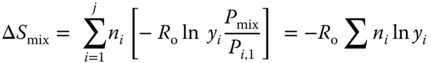
Consider two gases at the same initial temperature and pressure. If, after mixing, the mixture retains the same temperature and pressure, the associated entropy change is evaluated as follows:


Substituting for Pi,2 using the pressure fraction relationship and acknowledging isobaric conditions, this can be written as:
6.3.4 Thermodynamics of Mixture Separation
In a combustion process, carbon dioxide is generated in combination with other gases, i.e. in a mixture. In order to facilitate its capture and storage, it must first be separated from the other constituents. This will require the expenditure of work. The following analysis approaches the work evaluation from a thermodynamic perspective by first briefly considering the concepts of exergy, reversible work and irreversibility.
The work potential of a system is evaluated by the property exergy (X, kJ). It can be thought of as a measure of a system's thermomechanical state relative to its environment. A system existing at environmental conditions is often said to be in a dead state.
Energy is a property that is conserved according to the first law of thermodynamics. However, energy usage can result in the loss of some of the work potential.
In the everyday use of energy, exergy can be lost or destroyed by the presence of process irreversibilities such as heat loss, friction etc. Hence, exergy, unlike energy, is not conserved.
Reversible processes take a substance from its initial state to its final state in the absence of irreversibilities.
Work taking place in a reversible manner (Wrev) will be a maximum for a work production process and a minimum in a process requiring work.
If some useful work is involved, then the exergy destroyed is the difference between the reversible work and the useful work.
If a system changes to its dead state spontaneously, all of its exergy is destroyed.
For work production:
In an irreversible work‐generation process, the useful work (Wuseful) produced is less than the reversible work as a consequence of the presence of irreversibilities. Irreversibility can be described in terms of entropy change (ΔS), thus:
where To is a reference or environmental temperature.
Mixing of ideal gases is spontaneous and irreversible because work is needed to separate the components.
6.3.4.1 Minimum Separation Work
For an ideal, adiabatic mixing process, the entropy generated is equal to the change in mixture entropy and the exergy destroyed. Using Equations 6.17 and 6.19, the results of this argument are shown in Table 6.5 on molar and molar‐independent bases.
Table 6.5 Unit comparison of mixture entropy change and exergy destruction.
| Basis | Mixture entropy change | Units | Exergy destroyed in mixing | Units |
| Molar | kJ/K | kJ | ||
| Molar independent | kJ/kmol K | kJ/kmol |
For an ideal mixing process with no useful work generated, i.e. in the absence of irreversibilities, the reversible work is equal to the exergy destroyed. Applying the principle of reversibility, this must also be the minimum work input (Wmin,sep) for a mixture separation process.
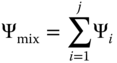
The minimum work of separation can be expressed in molar fraction, molar, molar flow (![]() or mass flow
or mass flow ![]() terms, with corresponding units as shown in Table 6.6.
terms, with corresponding units as shown in Table 6.6.
Table 6.6 Comparison of total separation work expressions.
| Basis | Work expression | Units |
| Molar independent (yi) | kJ/kmol | |
| Molar (ni) | kJ | |
| Molar flow ( | kW | |
| Mass flow | kW |
Note that the mass‐flow‐based expression in Table 6.6 was obtained by using the mass‐to‐mole converter, thus:
The above is applicable for the complete separation of components.
If separation is incomplete, the minimum work is determined by calculating the difference between incoming and outgoing mixtures.
6.3.4.2 Separation of a Two‐component Mixture
Let a gas mixture comprising two components A and B contain nA kmols of A and nB kmols of B. The corresponding mole fractions are yA and yB.
The minimum work of separation can be expressed in either mass or molar terms, with corresponding units as shown in Table 6.7.
Table 6.7 Comparison of two‐component separation work expressions.
| Basis | Work expression | Units |
| Molar independent (yi) | kJ/kmol of A | |
| Molar (ni) | kJ | |
| Molar flow ( | kW | |
| Mass flow | kW |
If the removal of one component (A) of a large mixture leaves the remaining mixture relatively unchanged, the minimum work required to remove A (kJ/kmol of A) is in molar terms, given by:
and in mass‐independent terms (kJ/kg of A):
The energy requirement will, of course, change as the removal proceeds because of the changes in mass and partial pressure.
A mass‐based estimate of the average energy requirement can be made by employing numerical integration (trapezoidal or the Simpson rule) between the process's start and end points.
6.4 Gas Separation Methods
6.4.1 Chemical Absorption by Liquids
Chemical absorption of CO2 is not a new technology. It already has applications in natural gas purification and the production of CO2 from gas turbine flue gases. These processes are, however, small scale when compared to the requirement of coal‐fired power stations.
Carbon dioxide can be removed from a flue gas mixture by washing or ‘scrubbing’ the mixture with a liquid sorbent or solvent that selectively binds chemically or reacts with CO2 in an absorber tower.
The gas‐loaded liquid is then pumped to a regenerator or ‘stripper’, where the gas is separated from the gas–liquid mixture by the application of heat.
The energy requirement for the process is solvent specific and is usually expressed as a percentage of the output of the power plant being treated.
The cleansed or lean solvent is recycled to the absorber for reuse.
The gas‐mixture regeneration process is not 100% efficient and some solvent make‐up is required. The take‐up of gas by the solvent is dependent on reaction kinetics (temperature, reactant concentrations) and, unlike physical absorption processes, is less reliant on gas partial pressure.
This method is therefore suitable for combustion process flue gas treatment where CO2 partial pressures are typically < 0.5 MPa.
Water will dissolve CO2 but, in order to improve reaction rates, substances with properties of both amines and alcohols dissolved in water are in common use as solvents in chemical absorbents.
Amines are hydrocarbons with one or more of the hydrogen atoms substituted by an ammonia (NH3) compound.
Alcohols are hydrocarbons with one or more of the hydrogen atoms substituted by a hydroxyl (OH) group.
Commercially available solvents include monoethanolamine (MEA), diethanolamine (DEA) and methyldiethanolamine (MDEA) in aqueous solution. Generically, these are termed alkanolamines. Solvent characteristics affecting CO2 absorption include solvent carbon chain length, the position of the alcohol/alkyl groups on the chain and whether the chain is open or cyclic.
A typical absorber/stripper plant schematic is shown in Figure 6.5.

Figure 6.5 Absorber/stripper plant layout schematic.
The flow inputs to the cycle are:
- The combustion flue gases to the absorber
- Make‐up solvent.
The flow outputs from the cycle are:
- De‐carbonized flue gases from the absorber
- Purified (>99%) CO2 from the condenser.
For an MEA system, the solvent typically undergoes the following changes:
- Unloaded solvent enters the absorber (∼40 °C) and experiences a small temperature rise (∼15 °C) by exit.
- The (carbon dioxide) loaded solvent leaving the absorber will be heated (by energy exchange with unloaded solvent leaving the stripper and further heated as necessary) before entering the stripper at high temperature (∼100 °C), where the solvent will be separated, leaving a carbon dioxide/water solution.
- The unloaded solvent leaving the stripper (∼90 °C) will be pumped to the absorber (being cooled by heat exchange with loaded solvent leaving the absorber and further cooling as necessary) to then re‐enter the absorber to complete its cycle.
The carbon dioxide/water exiting the stripper is dehydrated by a cooler/condenser.
6.4.1.1 Aqueous Carbon Dioxide and Alkanolamine Chemistry
Because of its ionic tendency, water is a good solvent and its hydroxide ion (OH−) can combine with aqueous carbon dioxide to produce hydrogen carbonate and carbonate ions, thus:
Alkanolamines react with water to form hydroxide ions.
Letting AANH be the generic formula for the alkanolamine:
Alkanolamines also react with the hydrogen carbonate ion to form carbamate ions, improving reaction rates and reducing equipment size.
6.4.1.2 Alternative Absorber Solutions
Alkali metal (Na/K) carbonates, chilled ammonia and amino acid salts have also being considered as alternative solvents with lower energy regeneration requirements.
The use of sodium and potassium carbonate solutions (Na2CO3, K2CO3) pre‐dates alkanolamines for CO2 chemical absorption applications.
The general reaction (for potassium carbonate) is shown below:
Again, carbonate ions are produced by the reaction.
The sodium/potassium hydrogen carbonate releases carbon dioxide when heated.
These resulting carbonates are again available for further CO2 take‐up. The advantage of using an alkali metal carbonate method is a lower energy requirement. Regeneration energy requirements are, in theory, less than for amine systems. However, having to operate with flue gases at higher pressure conditions (3 bar partial pressure of CO2 in absorber and desorption conditions of 3–4 bar total) would tend to negate this advantage.
Alkali metal methods also have a lower reaction rate and lower solubility. A compromise solution is to use alkali metal carbonates in tandem with DEA.
Ammonia is highly soluble in water:
Ammonia/CO2 chemistry is similar to that of amine/CO2 in its use of hydrogen carbonate, carbonate and carbamate ion formation.
The formation of carbamate ions is similar to that of alkanolamine solvents, with H2 replacing the generalized AA component. In general:
Other ammonia/carbon dioxide/water reactions are manifold, depending on reactant phase as well as temperature, pressure and concentration.
In ammonia‐based separation systems, the flue gases first require cleaning and cooling.
The absorber operates at temperatures slightly above 0 °C with desorption pressures of 15–20 bar. Ammonia recovery is via a wash cycle. Again, regeneration energy requirements are less than for equivalent amine systems.
Amino acid salts are also under consideration, as they possess, to some degree, all the advantages of amine, alkali salt and ammonia systems, in that they are basic, highly soluble in water and are able to form carbamates with CO2.
6.4.2 Physical Absorption by Liquids
Unlike chemical absorption, physical absorption relies on the ability of a liquid to dissolve a gas and the rate of (concentration‐difference‐based) diffusion from gas to liquid.
Henry's Law (named in honour of 19th century British chemist William Henry) is concerned with the solubility of a gas in a liquid and states that the mass of any gas (i) that will dissolve in a liquid at a constant temperature is directly proportional to the pressure that the gas exerts in contact with the liquid.
For a mixture of gases in contact with the liquid, the pressure of importance is the partial pressure contribution of the gas of interest.
The ‘law’ is, in fact, only an approximate relationship applicable to some gas–liquid solutions at low contaminant gas concentrations and equilibrium or saturation conditions (signified by *).
Furthermore, the relationship breaks down in the presence of gas–liquid ionization or chemical reaction. The law is commonly expressed thus:
where Pi is the partial pressure of the contaminant gas in the feed gas, y*i, g–l is the mole fraction of the gas in the liquid and KH is known as Henry's coefficient (Pa).
Each gas–liquid system has its own specific value of Henry's coefficient. Again, these values are temperature‐dependent. Raising the temperature reduces the liquid solvent's ability to hold the gas.
Dividing the above equation through by the total system pressure (Ptot), we have:
Using Dalton's Law, the left‐hand side of the equation becomes the mole fraction of the gas in the gas mixture associated with gas–liquid saturation conditions:
This mole‐fraction‐based expression is most commonly employed to illustrate the relationship in a gas–liquid absorption process. Care must be taken, as values of (KH/Ptot) are sometimes presented in standard texts in contrast to Henry's coefficient, KH.
Absorber/stripper systems are again used. As a consequence of Henry's Law, systems operate best with high‐pressure feed gases at CO2 partial pressures in excess of 0.5 MPa and system operating pressures of 1–10 MPa. Solubility and mass transfer can be optimized by providing a large interfacial contact area (i.e. tower packing), good mixing and sufficient contact time.
The solvent can be regenerated by a little heating or pressure reduction.
No chemical reactions occur, making the process stable and the energy requirement of regeneration lower than that for chemical absorption, as no chemical bonds need to be broken.
Water is a poor solvent for CO2 and so a variety of liquid solvents, principally alcohols, ethers and ketones, are used, including polyethylene glycol as well as methanol under a range of trade names.
Hybrid physical/chemical absorption liquids are also in use.
6.4.3 Oxyfuel, Cryogenics and Chemical Looping
The collection of carbon dioxide from flue gases would be made more tractable if the presence of other gases could be reduced.
Atmospheric air is approximately 79% nitrogen and 21% oxygen by volume. The nitrogen serves no useful purpose in a combustion process and formation of its oxides produces further pollutants (NOx).
Using pure oxygen in a stoichiometric hydrocarbon combustion process would produce carbon dioxide and water vapour only as products of combustion. The water vapour could be separated from the carbon dioxide by simple condensation. Carbon dioxide concentrations of 85–90% by volume in the resulting flue gas would then be possible.
This pre‐combustion processing of air is the essence of the so‐called oxyfuel process.
In practice, oxygen can be separated from air with a purity of 95–99%. The remaining few percent comprise some nitrogen and inert gases like argon.
Oxygen is produced on an industrial scale by cryogenic air separation. Air is compressed and cooled to about 93 K, at which point the oxygen condenses out. This is essentially a de‐nitrogenation process.
A standard power‐generation plant using the oxyfuel process will need modification. Due to the absence of nitrogen (which acts as a heat ballast), the use of pure oxygen raises the adiabatic flame temperature of the combustion process. Potential overheating is moderated by the recirculation of a fraction of the flue gases (see Figure 6.6).

Figure 6.6 Recirculation of flue gases in an oxyfuel combustion system.
Cooled flue gas recirculation to the burner may be needed to alleviate the problem in a retrofit situation. The burner may therefore be asked to operate in an oxygen/carbon dioxide/fuel environment. Optimization of burner design may be required, with excess oxidant implications.
However, with increased temperature come a lower heat exchange area, smaller size and cost savings.
Boiler plants lend themselves to retrofit more readily than gas turbine systems.
However, oxygen production comes at a price. Current estimates are that the oxyfuel system can consume up to 25% of a plant's electrical energy production, perhaps reducing plant efficiency by up to 10%. Much research is being carried out to produce an oxygen separation method with a reduced energy demand. Candidates include species‐selective membranes and chemical sorbents.
Chemical looping combustion (CLC) is another pre‐combustion process based on the ability of a metal (e.g. nickel, cobalt, copper, iron or manganese) to be readily oxidized in the presence of atmospheric oxygen and to release its oxygen, i.e. be reduced, in the presence of the fuel. A schematic is shown in Figure 6.7.

Figure 6.7 Chemical looping system.
Denoting the metal M, in the air reactor:
In the fuel reactor:
The metal oxygen carriers take the form of 0.1–0.5 mm particles. The reactor typically takes the form of a circulating fluidized bed, typically operating at a temperature of around 1000 °C.
The search is on for oxygen‐carrying materials with good oxygen transfer capacities, high reactivity and rapid take‐up. Other desirable characteristics include low fragmentation, low attrition and a low tendency to agglomerate. Low toxicity is also, of course, desirable.
Operational experience of CLC plant utilizing natural gas with a capacity of up to 50 kW was available around ten years ago. Some plant experience with solid fuel and syngas has become more available since 2010. So far, more than 900 suitable oxygen‐carrying materials have been identified and about 30 (for example, NiO, Fe2O3, CuO, CoO) have been tested in practice.
6.4.4 Gas Membranes
Gas membrane technology is over 50 years old. Membranes separate gases by virtue of the presence of small pores or sorption and diffusion.
Carbon dioxide can be separated from a mixture of gases by exposing the mixture to a barrier or membrane that is selectively permeable to CO2.
Current membrane technology is not as capture effective as absorption or cryogenics, and resulting CO2 purities are inferior to these technologies. Membrane lifetimes are of the order of 3–5 years. However, energy requirements can be lower than for other technologies.
The driving force for separation is upstream ( feed) to downstream (permeate) membrane partial pressure difference for the CO2. Target gas remaining in the feed stream is often termed retentate.
6.4.4.1 Membrane Flux
As mentioned, the transport mechanisms through membranes are solution and diffusion or permeation through the empty space of the membrane.
Defining SA as a solubility coefficient (m3(STP)/m3. m. Pa) of the gas (A) to be separated and DA as the diffusion coefficient (m3/s) or molecular mobility for the membrane, the permeability of the membrane to gas component A is given by the product:
The term permeance (m2/s. Pa) or molecular conductance of the filter to gas (A) is also in use and is given by:
where L is the membrane thickness (m).
Clearly it is desirable to maximize this parameter by choosing a membrane material with a high permeability at the minimum membrane thickness possible commensurate with other operational conditions.
The volume flow rate per unit area of the membrane or flux![]() of component gas (A) through the membrane is then given by:
of component gas (A) through the membrane is then given by:
where PA is the partial pressure of the gas (A) to be separated.
A further membrane characteristic called the selectivity is in common use.
In a system with two gases this is defined as the ratio of the target gas permeability to the unwanted gas component permeability.
6.4.4.2 Maximizing Flux
Low permeance can be overcome by increased membrane area, and low values of selectivity can be overcome with multi‐staging or cascading of membranes.
Looking at the flux relationship, the rate of transfer could also be increased by increasing the partial pressure of the target gas on the feed side of the membrane and/or lowering the partial pressure of the target on the permeate side (i) or by applying a vacuum (ii) or by sweeping the permeate side with an inert gas (iii) (see Figure 6.8).
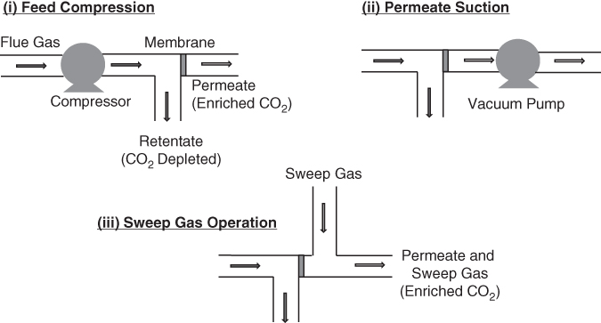
Figure 6.8 Membrane partial pressure enhancement strategies.
6.4.4.3 Membrane Types
Membrane types can be divided into polymer and inorganic varieties.
6 Polymer (Polymeric) Membranes
Polymer membranes used for pre‐ and post‐combustion applications can be subdivided into polyimides, facilitated transport, mixed matrix and poly‐ether‐oxide (PEO) types.
Polyimides make good separation membranes because, in addition to a high selectivity and permeability for CO2, they have a high thermal stability, good chemical resistance, mechanical strength and good electrical characteristics.
Facilitated transport membranes contain a metal ion carrier to chaperone a gas selectively across the barrier. Problems with carrier degradation leave a question mark over their use with coal‐fired plant.
Mixed matrix membranes (MMMs) have a micro or nanoparticle inorganic material as part of a polymer matrix. At present, these types display only moderate separation performance due to poor interfacial adhesion between matrix and inorganic component. Higher thicknesses are required, leading to a low flux.
Poly‐ether‐oxide (PEO) membranes have increased performance as a consequence of the polarity of the ether oxide presence. Good CO2/N2 selectivity and high CO2 permeance have been reported.
6 Inorganic Membranes
Inorganic membranes use either (conductive) metals or ceramics as a selective barrier.
Metallic membranes tend to be described as dense. Palladium and its alloys are in use as membrane materials.
Ceramic membranes can be either dense or microporous. Dense ceramic membranes are used to facilitate either oxygen separation using ionic/electronic transfer (800–1000 °C) or hydrogen separation using protonic/electronic transfer (500–800 °C). Microporous membranes can be further subdivided into crystalline types (e.g. zeolites) and amorphous types. Structurally microporous membranes are graded. The smallest pore sizes need to be very small, as the diameters of gas molecules are typically less than 1 nm across and have a narrow range of values, for example, carbon dioxide 0.33 nm, hydrogen 0.289 nm, oxygen 0.346 nm and nitrogen 0.364 nm.
Operating temperatures for ceramic membranes are much lower (< 400 °C).
Both dense and microporous types are suitable for pre‐ (H2/CO2) and post‐ (CO2/N2) combustion separation.
6.5 Aspects of CO2 Conditioning and Transport
The capture of carbon dioxide may take place at large power‐generating plants that are remote from the final destination CO2 storage site, and so a large network of CO2 pipelines along with integrated truck/ship transportation may be required. Carbon dioxide pipeline transportation technology is not new, and there is already operating experience albeit for a different reason.
For example, the USA has a CO2 network of several thousand kilometres that utilizes naturally occurring geological reservoirs of CO2 for enhanced oil recovery (EOR) in oil fields. The CO2 (often along with water) is pumped into depleting oil fields to maintain pressure at depth to keep oil production at an acceptable level. Pipe diameters are typically less than 1 m.
Dedicated CO2 pipelines performing the same function can also be found in Algeria, Canada, Hungary and Turkey.
However, the issues associated with this provision in the carbon sequestration chain are many.
6.5.1 Multi‐stage Compression
Carbon dioxide is usually transported in a liquid or supercritical condition.
The advantages of the supercritical condition are a high density (smaller pipes) and a low viscosity (lower pressure drop/km).
In all cases, the occurrence of two‐phase (gas/liquid) flow is to be avoided, as this can result in increased energy pumping costs and possible pipeline damage due to cavitation. For this reason, a minimum pressure above critical conditions (73.9 bar) is maintained in existing pipelines.
Minimizing the work input or energy associated with CO2 pressurization is important. The work input to a compression process will be minimized when irreversibilities, for example, heat losses, friction, noise etc., are minimized. The (internally) reversible work input will then be given by:

The minimum work could be achieved by employing an excruciatingly slow compression, but it is more practical to minimize the specific volume by keeping the gas temperature as low as possible during compression. The ideal case would then be an isothermal compression.
A comparison of an isothermal compression process (max cooling, index of compression 1) with an isentropic compression process (no cooling, index of compression k) and a polytropic compression process (some cooling, index of compression, 1 < n < k) assuming perfect gas conditions is shown in Figure 6.9.

Figure 6.9 Comparison of gas compression (1–2) processes.
Remember that the work of compression is the area under the curve on a P–v diagram.
The work (kJ/kg) expressions associated with each process are:
- Isentropic:
(6.30)

- Polytropic:
(6.31)

- Isothermal:
(6.32)

For a single‐stage compression, a cooling jacket around the compression cylinder may be sufficient, but for multi‐stage systems, constant pressure intercooling between stages is employed, with the fluid being cooled to the compressor inlet temperature.
Although real compression processes are usually regarded as polytropic, intercooling and staging do reduce the work input, as shown in Figure 6.10.

Figure 6.10 Gas compression with intercooling.
The total work for a two‐stage polytropic compression process (index of compression n) is given by:

where Px is the intermediate pressure and T2 is the temperature of the gas entering the second stage. Note that with perfect intercooling between stages, T1 = T2.
The work saved is a function of the intermediate pressure. The optimal intermediate pressure that minimizes the work input and maximizes the work saved can be determined by differentiating the above expression with respect to Px and setting the result to zero. This gives:

Typically, the CO2 is pressurized in a multi‐stage process to just above critical pressure (∼80 bar) and pumped up to the transport pressure (∼150 bar). A typical dehydration/pressurization string comprising a heat exchanger (HX) or cooler, water separator (S) and compressor (C) is shown in Figure 6.11.

Figure 6.11 Dehydration/pressurization cascade.
6.5.2 Pipework Design
6.5.2.1 Pressure Drop
A significant drop in pressure will occur over long pipe lengths. It is undesirable for the pressure changes to result in two‐phase conditions and so pumping stations will be required along the length of the line.
Pressure losses for single‐phase flow can be approximated using a range of standard techniques but will generally depend on pipe diameter and material, CO2 density and viscosity and flow rates and velocities. Because of the high‐pressure operating environment, increased pipe thicknesses are specified.
6.5.2.2 Materials
Carbon dioxide forms carbonic acid with water, but if the CO2 is dry then carbon steel pipes are suitable. Large temperature reductions can occur under depressurization and so pipes must also be fracture‐resistant.
Seal/gasket material selection should be given special consideration, as standard elastomers absorb CO2 and swell, resulting in potential failure.
Plastics such as PTFE, PP and nylon are generally suitable for use with CO2.
Hydrocarbon‐ and fluorocarbon‐based lubricants are used with CO2 systems.
6.5.2.3 Maintenance and Control
Pipelines are monitored at intervals and controlled centrally with respect to pumping speeds, valve operation, leak detection, flow rate measurement etc.
Flow measurement and metering techniques include orifice and vortex types.
The internal pipe conditions can be monitored with the use of pigs performing a cleaning function as well as checking for internal corrosion and mechanical deformation.
Pipelines should also be designed with sufficient isolation, emergency shut‐off and blow down valves.
For smaller quantities of CO2, ship transport is also an option. In this case, the CO2 is usually transported as a chilled liquid.
Current CO2‐dedicated ship transports are few and small in capacity (typically 1000–1500 m3). There are a few larger vessels with a capacity of up to 10 000 m3 certified to carry CO2. Transport pressures of up to 20 bar are used.
6.5.3 Carbon Dioxide Hazards
6.5.3.1 Respiration
Inhaled (atmospheric) carbon dioxide has a concentration of about 0.04%. The partial pressure of carbon dioxide in the blood is higher than this (1.4%) and so CO2 can diffuse out of the blood to be exhaled. If the concentration in inhaled air increases above this level, carbon dioxide cannot be released from the blood. In fact, further CO2 may be absorbed, increasing blood acidity. The involuntary response may be to take longer/deeper breaths, exacerbating the situation.
The time‐dependent physiological effects of increasing ambient CO2 concentration (%) are divided into four categories of increasing severity. For example, at an exposure time of around 20 minutes, indicative effects at associated ambient concentrations (%) are as follows:
- 0–1% – no noticeable effect
- 1–4.5% – small hearing loss, doubling in depth of respiration
- 4.5–7.5% – mental depression, dizziness, nausea
- >7.5% – dizziness, stupor, unconsciousness.
- Exposure limits in the UK are set by the Health and Safety Executive. Current values (see www.hse.gov.uk/carboncapture/carbondioxide.htm) are:Long term (8 hr) – 5000 ppm, i.e. 0.5% CO2
- Short term (15 min) – 15 000 ppm, i.e. 1.5% CO2.
6.5.3.2 Temperature
If gaseous carbon dioxide experiences a sudden drop in pressure, cooling will result. Carbon dioxide snow may be formed, causing cold burns when coming into contact with skin or eyes.
6.5.3.3 Ventilation
In the event of a leak, high concentrations of CO2 can build up quickly in confined spaces. For example, the specific volume of liquid CO2 will increase by approximately 800 times on evaporation.
The molar mass of CO2 is greater than air, hence carbon dioxide will tend to accumulate at low levels in an unventilated, still air situation. Detection equipment and low‐level exhaust louvres are necessary in such spaces and around plant.
Due to the reduction in temperature associated with a pressure drop, contaminants such as water may also condense, forming fogs. Although useful in indicating a leak, they are no indication of resulting CO2 concentration.
6.6 Aspects of CO2 Storage
Storage of carbon dioxide in pressure vessels is out of the question because of the magnitude of annual CO2 combustion‐associated release. However, Nature has been practising carbon capture for quite some time, and enhancing these techniques provides at least a direction for solving the CO2 emission problem.
6.6.1 Biological Sequestration
In 1660, Flemish chemist Jan Baptista van Helmont started to grow a willow tree in a pot. After five years the tree weighed about 70 kg while the soil had only lost about 30 g in mass. He concluded that the soil matter (mostly aluminium silicates) was largely irrelevant to the growth of plants other than to provide mechanical support and act as a water‐storage vessel.
The soil water, of course, is vital in itself and as a medium for the supply of very small amounts of dissolved inorganic substances needed by plants.
Even the supply of water does not provide the whole story. Living matter contains much carbon but there is insufficient carbon in soil to account for plant growth.
As fate would have it, van Helmont had also conducted mass balance experiments on the burning of charcoal. He noted that the post‐combustion ash weighed less than the fuel, and came to the conclusion that some wild spirit or gas had been formed to account for the mass difference.
In 1727, English physiologist Stephen Hales determined that atmospheric carbon dioxide was the source growth material that van Helmont had been looking for.
In the 1770s, English minister Joseph Priestly carried out some simple experiments with a bell jar. First, he attempted to grow a plant under a bell jar with a limited supply of carbon dioxide. He noted that even if water and sunlight were plentiful, the plant would grow no more once its supply of CO2 was exhausted. Next, he placed a mouse under a bell jar and noted that it would expire when its supply of oxygen (O2) had been exhausted. Finally, he placed a mouse and a plant under a bell jar together and noted that they would continue to survive for longer than each did in isolation. From these results, he correctly reasoned that plants on land (and in the oceans) consumed carbon dioxide and released oxygen while animals consumed oxygen and gave off carbon dioxide.
The significance of this was not lost on Dutch physician Jan Ingenhousz, who, in 1779, published one of the earliest books on ecology and material balances in the environment. His ideas about carbon dioxide, oxygen and water utilization and reformation became crystallized by the phrase photosynthesis, meaning ‘manufactured by light’.
Photosynthesis is a widely used term to describe how green plants use carbon dioxide, water and sunlight to manufacture carbohydrates (or starch). A simple equation describing this process is given below:
In the 19th century, work was done on determining which characteristics of plants facilitated this process. Attention was focused on what made plants green, as this colouration is uncommon in animals. In 1819, two French chemists, Pierre Joseph Pelletier and Joseph Bienaime Caventou, succeeded in extracting a green pigment called chlorophyll (meaning ‘green leaf’). They determined that chlorophyll is, in fact, a catalyst.
The structure of chlorophyll was not established until the early part of the 20th century, when two German chemists, Richard Wilstatter and Hans Fischer, determined its composition.
Chlorophyll has a complex structure with a number of variants, but essentially it comprises a ring‐shaped head with a magnesium atom (Mg) at its centre bonded to four nitrogen atoms. The head is connected to a long hydrocarbon molecule ‘tail’, known as a carotenoid (see Figure 6.12).

Figure 6.12 Structure of chlorophyll.
The substance appears green because it absorbs the red, orange and blue wavelengths (450–670 nm) of light whilst reflecting the remainder. These longer wavelengths contain less energy than light at the blue end of the spectrum but are able more easily to penetrate the dust and gas of the atmosphere. The solar energy absorbed by the chlorophyll raises its electrons from their ‘ground’ state to an elevated level. On return to the ground state, the energy is made available to facilitate chemical reactions.
These reactions were first discovered by experiments with isotopic tagging using heavy oxygen (O18). The work was carried out by two American biochemists, Samuel Ruben and Martin D. Kamen. They determined that it was the water molecule that was split up into hydrogen and oxygen during photosynthesis. Photosynthesis is therefore concerned with the photolysis, or breaking down, of water.
The split oxygen and hydrogen components of the water can have two possible futures. Half of the hydrogen takes part in the so‐called respiratory chain, generating three molecules of a chemical energy store called adenosine triphosphate (ATP) to be reunited later with some of the oxygen to form water. The remainder of the hydrogen combines with the carbon dioxide to form carbohydrates. This is facilitated by the presence of a five‐carbon sugar molecule, ribulose bisphosphate (RuBP), found in plant cells. This process is energy consuming and utilizes the previously manufactured ATP. Oxygen is not used in this latter process and is released to the atmosphere. This is summarized in Figure 6.13.

Figure 6.13 Simplified schematic of photosynthetic pathway.
In this way, land‐based and oceanic plants have been extracting atmospheric CO2 for millions of years. Clearly, not destroying existing planetary forestation and vegetation and enhancing and encouraging replanting will help. However, it is widely believed that this approach cannot alone supply a carbon sink sufficient to compensate for anthropogenic combustion activity.
6.6.2 Mineral Carbonation
Carbon dioxide has an affinity to combine with some light metal oxides like magnesium and calcium to form solid metal carbonates, for example:
The reaction is exothermic, i.e. it releases heat rather than requiring it.
Simple light metal oxides are rare in the lithospheric environment and these metals are more commonly found in silicate combinations such as in the minerals forsterite (Mg2SiO4) and serpentine (Mg3Si2O5(OH)4).
These, too, however, will combine with carbon dioxide, thus:
The resulting carbonate products are stable and do not re‐release the captured CO2. This is in contrast to other carbon storage options where leakage is a possibility.
These reactions have, therefore, been proposed as the basis of a carbon capture and storage solution, since the raw material magnesium‐rich rocks are relatively common and close to the surface, making their extraction relatively simple.
However, resulting from the prevailing reaction kinetics, simply exposing carbon dioxide to rocks directly would be an unacceptably slow process and, in practice, the rock would need pre‐treatment in the form of crushing and the addition of a solvent to precipitate out the desired minerals.
The solvation itself presents problems, as current solvent candidates include hydrochloric acid, molten magnesium chloride salts and water. Using an acid solvent is an energy‐hungry process, requiring the removal of large quantities of water. The molten salt option brings corrosive problems to the process. Using water (enhanced with Na2CO3) as a solvent is, on the face of it, less environmentally aggressive but is slow and still energy‐intensive.
To date, therefore, all mineral carbonation processes would impose a significant parasitic effect on the energy produced by the target power station.
Due to low overburden and the presence of comparatively thick mineral‐bearing strata, the mining cost of metal silicates appears to be low. It has been estimated that typically around 8 tonnes of magnesium silicate ore would be needed to capture and store the carbon dioxide released by 1 tonne of coal.
The infrastructure needed to transport such large quantities of raw material to a distant power station would be significant, and it has been proposed that, if this technology can be made economic, the capture process be carried out at the mineral source mine with storage on site. For minimum impact, the CO2 generator would, of course, then be sited adjacent to the mineral mine.
6.6.3 Geological Storage Media
Geological or fossil CO2 is found in rocks at a number of sites around the world, for example, Mexico, the USA, Hungary, Turkey and Romania.
CO2 is also very commonly associated with oil and natural gas reservoirs. Indeed, there are so‐called low‐BTU gas fields in the USA and Asia comprising mostly CO2 in association with some methane and low levels of other gases like H2, SOx, N2 and C3H8.
This occurrence would indicate that one way forward for large‐scale carbon dioxide storage is to inject the gas into suitable rock strata.
At the time of writing, attention is focused on porous media such as depleted oil and gas reservoirs and deep saline rocks.
The important characteristics for a potential porous store are:
- Local and regional geology – long‐term tectonic stability.
- Presence of an impermeable, continuous overlying or ‘cap’ rock.
- Storage dimensions and porosity – dependent on overall vertical and horizontal dimensions.
- Storage pressure – flow rate into (injectivity) and through (permeability) the store.
Carbon dioxide is best injected in its supercritical condition to provide a high density associated with a low viscosity.
The supercritical pressure (>7.3 MPa) can be maintained at depths of about 800 m.
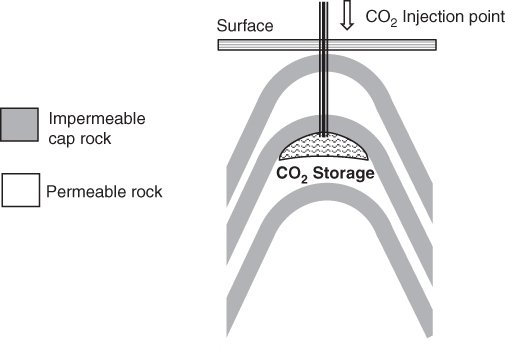
Figure 6.14 Example of structural trapping in an anticline.
Geological trapping can be subdivided into structural, stratigraphic, solubility, residual and adsorption forms.
- Structural trapping relies on the presence of an impermeable cap rock to halt the upward migration of the CO2. This can be provided by the presence of anticlinal (arch‐shaped) or faulted (slipped) rock formations (see Figure 6.14).
- Stratigraphic trapping relies on changes in the porosity and permeability characteristics within a given rock stratum.
- Solubility (or dissolution) trapping relies on the CO2 dissolving into the existing rock fluids. The solubility depends on pressure, temperature, contact area and composition of the inherent solvent.
- Residual trapping is based on the drainage‐imbibition process. In this phenomenon, the carbon dioxide will displace the existing strata fluids (brine or hydrocarbons) but only if the injection pressure is maintained. After this ceases, the displaced fluid attempts to return to the rock, thus encasing the CO2 and forming a seal around the gas. The process depends on the rock pore capillary forces.
- Adsorption trapping of CO2 storage in coal seams relies on the adsorption of the gas, displacing the in situ methane from pores within the rock. The process is reliant on concentration‐dependent diffusion. It has been determined that the suitability of a coal seam for storage is dependent on a number of factors including:
- ➢ Coal carbon and volatile content.
- ➢ Temperature: Adsorbed gas decreases with increasing temperature.
- ➢ Water content: Adsorbed gas decreases with decreasing water content.
- ➢ Ash content: Adsorbed gas decreases with increasing water content.
- ➢ Desorbed gas composition.
- Salt domes (see Figure 6.15) provide another option for geological gas storage. Salt domes are essentially column‐shaped aquifers (containing non‐potable water or brine in their pores) that have deformed and intruded into overlying layers. They generally comprise sodium chloride with some calcium sulphate.

Figure 6.15 Salt dome CO2 storage.
Pumping water into the formation has a leaching effect and creates cavities suitable for gas storage.
The technology is not new and was deployed first (France, Germany, South Africa and the USA) in the 1970s to store natural gas and oil during the energy crises.
If the walls of the dome are impervious, the system can be leak‐tight.
A crude estimate of the CO2 storage capacity (![]() , kg) of a geological feature is given by:
, kg) of a geological feature is given by:
where ηstorage is a measure of the injection effectiveness. Typical efficiencies range from 2–40%.
6.6.4 Oceanic Storage
The oceans cover an area of approximately 362 × 106 km2, i.e. 71% of the earth's surface, and provide a habitat for about 80% of the planet's life.
The average depth of the oceans is about 4 km. This compares with an average height above sea level of less than 1 km for the land masses. At the deepest point, in the Marianas Trench in the Pacific Ocean, the land falls away to more than 11 km.
Typically, the breakdown by volume for dissolved gases in the ocean indicates a reduced nitrogen content and an increase in oxygen and carbon dioxide presences compared to atmospheric air. Reported values vary.
Although surface waters are often saturated with atmospheric gases, Henry's Law is of limited use in modelling actual hydrospheric conditions in deep water. Here, conditions are usually determined by measurement.
The distribution of dissolved gases in the ocean is uneven, having a layered structure linked to winds, waves, oceanic currents and biological activity such as photosynthesis, respiration and decomposition.
Levels of carbon dioxide are at a minimum of about 60–70 mg/litre at the surface, due to consumption by marine plants in photosynthesis, and increase to a maximum value at around 1000 m depth due to respiration and decay generally.
Carbon dioxide dissolved in water generates ions. The addition of carbon dioxide to oceanic water therefore increases its acidity:
As a consequence of anthropogenic activity and related atmospheric carbon dioxide concentrations, it is estimated that the planet's oceanic surface water pH value has decreased (i.e. acidity has increased) by 0.1 to under 8.1 since the beginning of the Industrial Revolution. Notwithstanding this, the ocean has been suggested as a potential store for the direct injection of CO2 emissions.
Predicting the state of carbon dioxide is dependent on knowledge of its pressure and temperature. The pressure and temperature conditions in the ocean, i.e. the CO2 containment vessel, vary markedly.
Water pressures in the oceanic hydrosphere vary from zero (gauge) at a free surface to over 100 MPa at great oceanic depth, i.e. approximately 1000 × that found at sea level (∼1 × 10⁵ Pa). The exact pressure–depth relationship in deep water is, however, nonlinear due to changes in composition and, at great depth, some slight compressibility effects.
The oceanic hydrosphere is, in some instances, heated by a range of local, high‐intensity temperature sources such as volcanoes, hot springs etc. For example, local water temperatures of up to 400 °C have been found at hydrothermal vents on the sea floor.
However, the main source of energy input, especially for open bodies of water, is solar radiation. Solar radiation at the earth's surface is a diffuse form of energy. Average oceanic surface temperatures are typically 18 °C, with a range of −2 to 36 °C.
Over its entire volume, however, the ocean is a relatively cold place, with its average temperature in the range of 3–4 °C. Global ocean temperatures vary with latitude and depth, largely due to differences in solar energy input and wave/current action. The coldest water is at the poles; the warmest between the tropics.
With this in mind, CO2 oceanic injection points at depths of less than 500 m result in the CO2 existing in its gaseous form.
At depths of between 500 m and around 2700 m, the CO2 will exist as a liquid but will be positively buoyant, i.e. it will have a tendency to float up, being less dense than the surrounding seawater.
Below 2700 m, the CO2 will be more dense than the surrounding seawater and will be negatively buoyant, i.e. it will tend to sink.
In addition to gaseous and liquid carbon dioxide, a third state is of interest – the solid CO2 hydrate. Carbon dioxide hydrates are created when the hydrogen bonds of adjacent water molecules form a framework with a central cavity occupied by CO2 molecules. The attraction of this exotic structure is its stability, negative buoyancy and its ability to promote dispersion. It is, however, at present difficult to produce, requiring relatively low temperatures (∼10 °C) and high pressures.
Current suggested methods of CO2 release into the ocean include forming either CO2 lakes on the oceanic floor (>3000 m) or CO2 plumes within the oceanic body itself. Both shore‐sourced pipelines and ship transport/offshore delivery systems are being considered.
Whatever the chosen method, the CO2 is not permanently isolated from the atmosphere and, over time (several centuries), the gas will be liberated and reunited with the atmosphere via the ocean surface. However, it is hoped that man‐made release of carbon dioxide will have abated by that time.
In terms of environmental impact, the effects on marine organisms of the increase in CO2 oceanic water concentrations and attendant lowered pH values associated with direct injection are under intensive study.
6.7 Worked Examples
Data for use in the following worked examples:
- Universal gas constant: Ro = 8.314 kJ/kmol K
- Molar mass of carbon dioxide:
 = 44 kg/kmol
 - Molar mass of nitrogen:
 = 28 kg/kmol
 - Carbon dioxide (CO2) critical point properties: 73.9 × 10⁵ Pa, 304.2 K
- Nitrogen (N2) critical point properties: 3.39 MPa, 126.2 K.
6.8 Tutorial Problems
Use the following properties where appropriate:
- Universal gas constant: Ro: 8.314 kJ/kmol K
- Molar masses: CO2: 44.01 kg/kmol N2: 28 kg/kmol
- Molar specific heat capacity at constant volume: CO2: 28.9 kJ/kmol K N2: 21 kJ/kmol K
- Specific gas constant for CO2: 188.9 J/kg K.
- 6.1
Predict the pressure (MPa) of carbon dioxide (CO2) at a temperature of 40 °C and a specific volume of 0.011939 m3/kg using:
- The perfect gas law.
- Van der Waal's equation.
- The Beattie–Bridgeman equation.
- The Benedict–Webb–Rubin equation.
[Answers: 4.955 MPa (+23.9%), 4.072 MPa (+1.8%), 3.981 MPa (−0.4%), 4.043 MPa (1.0%)]
- 6.2 A gas mixture comprises 10 kmol of CO2 and 2 kmol of N2. Determine the mass (kg) of each gas and the apparent gas constant (kJ/kg K) for the mixture. [Answers: CO2 – 440 kg, N2 – 56 kg, 0.202 kJ/kg K]
- 6.3 A gas mixture comprises 7 kg of CO2 and 2 kg of N2. Determine the pressure fraction for each gas and the apparent molar mass of the mixture (kg/kmol). [Answers: CO2 – 0.69, N2 – 0.31, 39.04 kg/kmol]
- 6.4
Determine the reversible work (
 ) associated with the removal of carbon dioxide having a molar fraction of 0.1 in a gas mixture at a temperature of 120 °C. [Answer: 170.94
  ]
] - 6.5
Carbon dioxide at 1 bar pressure and 20 °C is to be compressed to 9 bar. Determine the work of compression (kJ/kg) if the compression is carried out by:
- A single‐stage isentropic process (k = 1.287).
- A single‐stage polytropic process (n = 1.2).
- A single‐stage isothermal process (n = 1).
- A two‐stage polytropic compression process (n = 1.2) with an intermediate pressure of 3 bar and perfect intercooling, i.e. the gas enters the second stage of the compression at 293 K.
- 6.6 Carbon dioxide is to be compressed from 1 bar to 16 bar in a two‐stage process. What is the optimal intermediate pressure for this process? [Answer: 4 bar]
- 6.7
It is proposed that elemental iron (MFe = 56 kg/kmol) is to be used as the oxygen carrier in a chemical looping combustion system using coal (modelled by elemental carbon MC = 12 kg/kmol). Using the simple fuel reactor equation, determine the approximate mass of iron (tonnes) required to burn 1 tonne of coal. Give a reason why the amount of iron required, in practice, would be in excess of that indicated by the calculation.
[Answer: 9.33 tonnes Fe, excess air]
- 6.8
Assume the production of carbohydrate (starch) by green plants is governed by the simplified equation below:
Determine approximately how much CO2 (ktonne) would be absorbed in the manufacture of 1 ktonne of starch and how much O2 (ktonne) would be evolved.

[Answers: 1.47 ktonne CO2, 1.07 ktonne O2]
- 6.9
It has been suggested that the mineral serpentine (Mg3Si2O5(OH)4) be used to capture the carbon dioxide from a power plant emitting 5 Mt per annum. Determine the amount of serpentine (Mt/annum) and the percentage breakdown by mass of the reaction's products.
[Answers: 10.45 Mt, 61.8% MgCO3, 29.4% SiO2, 8.8% H2O approximately]
- 6.10 A rock stratum having an area of 250 × 106 m2, a thickness of 150 m and a porosity of 20% is selected as a potential CO2 store. The CO2 storage gas density is to be 700 kg/m3 and the storage efficiency is predicted to be 40%. Determine the storage capacity (kg) and what percentage of an annual global CO2 emission of 36 Gtonne could be accommodated by the store. [Answers: 2.1 × 10¹² kg, 5.8%]