8
Alternative Energy and Power Plants
8.1 Overview
Global warming is one of the most serious challenges facing humanity today. It has come about partly due to the consumption of electricity, partly due to the burning of fuel for heating and transport and partly due to the increase in global human and livestock populations. Its impacts adversely affect all aspects of the natural world. To protect the health and economic well‐being of current and future generations, we must reduce our emissions of greenhouse gases by using the technology, know‐how and practical solutions already at our disposal. In particular, it has been proposed that the world's electrical power demands from coal must fall and be replaced by a renewable fuel such as solar, wind, bioenergy or hydropower.
There is a unified international agreement to limit the use of fossil fuels and to adopt renewables to cover some of our demands for power and heating. For example, in Europe, the EU20‐20 accord is an attempt to source 20% of energy consumption from renewables by the year 2020.
The recent and projected growth for global electrical energy generation (1990 to 2040), as predicted by the US Energy Information Administration, is shown in Figure 8.1.

Figure 8.1 World electricity generation 1990–2040. Data courtesy of EIA 2013 report.
This chapter describes some of the alternative, non‐fossil‐fuel energy technologies, including the non‐renewable nuclear option, available to combat global warming and meet these objectives.
8.2 Nuclear Power Plants
Currently, nuclear power produces approximately 17% of global electricity. The contribution varies from country to country. In France, over 75% of electricity is produced by nuclear power. The United States and the United Kingdom, on the other hand, only produce about a quarter of their electricity from nuclear fission.
Nuclear fission is the splitting of an atom's nucleus, by a neutron, into lighter nuclei, electrons and further neutrons and perhaps electromagnetic radiation.
Fission‐sourced neutrons can be captured by other adjacent atoms to continue the (chain) reaction. In the presence of sufficient nuclear material, the reaction becomes self‐sustaining.
Nuclear fission also produces heat as a by‐product, and this heat can be used to make steam for use in a conventional power cycle. Hence, aside from the heat‐generation method, nuclear power generates electricity much like a coal‐fired power plant but without the associated carbon dioxide emissions. Like their fossil‐fuel counterparts, nuclear power plants can also be a huge source of thermal energy for heating, if required.
Due to the difference in the binding energies of the parent atom and its fission products, the nuclear fission of a single uranium‐235 nucleus can produce up to 200 MeV or 3.2 × 10⁻¹¹ J of energy. This approximates to 82 TJ/kg and is quite impressive when compared with that of 34 MJ/kg for an anthracite coal.
8.2.1 Components of a Typical Nuclear Reactor
A nuclear reactor consists of a vessel with fuel rods, control rods, the moderator and a coolant.
Reactor fuel rods are commonly made of uranium oxide.
Control rods are made from a material (for example, boron, cadmium, hafnium) with good neutron‐absorbing capabilities, useful in regulating or shutting down the reaction.
The moderator is a material (for example, graphite or water) surrounding the fuel rods that is used to slow down generated neutrons to a speed or energy conducive to capture by uranium nuclei.
The coolant is a fluid (for example, water, CO2, liquid sodium) used to collect the thermal energy generated by the reactor.
A containment structure prevents radioactivity from escaping to the environment.
8.2.2 Types of Nuclear Reactor
Water reactors can be of the pressurized‐water or boiling‐water variety.
In a pressurized‐water reactor, the thermal energy of the nuclear reaction is used to heat a primary coolant circuit that produces steam in a secondary circuit via an indirect heat exchanger (see Figure 8.2). The steam is then routed to the turbine set for power production.

Figure 8.2 Pressurized‐water reactor (PWR).
In a boiling‐water reactor, the indirect heat exchanger and secondary circuit are dispensed with and power is generated by sending steam directly to a turbine.
8.2.3 Environmental Impact of Nuclear Reactors
Although proponents of nuclear power often emphasize the carbon‐free aspect of the technology, all forms of radiation, whether man‐made or naturally occurring, are potentially dangerous, and therefore nuclear power is not without its own radioactive waste issues.
Nuclear power waste is commonly classified into:
- High level – spent reactor fuel, reprocessing material.
- Intermediate level – reactor ancillary equipment, e.g. control rods, instrumentation etc.
- Low level – contaminated laboratory material, operator clothing, miscellaneous rubbish.
During its passage through matter, radiation knocks electrons out of atoms or molecules (ionization). There is no known lower limit of radiation below which no damage is done to living tissue, and the human species is more sensitive than most to radioactivity. Some forms of radioactivity are persistent, having a high mobility in the environment and a tendency to concentrate in biological systems.
Radiation damage takes three forms: immediate physical damage to tissues (‘radiation burns’); delayed damage (cancer); and genetic abnormalities (mutations) including cancer in successive generations.
There are three common SI units describing the effects of radioactive emission/absorption:
- Becquerel – Quantifies the emission rate or activity of a radioactive source.
- Gray – An absorbed dose of radioactive energy (J/kg of tissue).
- Sievert – An absorbed dose modified by a factor to account for the relative susceptibility of the irradiated tissue to a particular type of ionizing radiation, e.g. alpha particles, beta particles, gamma rays etc.
8.3 Solar Power Plants
The sun is an enormous nuclear fusion reactor around which the earth orbits at a distance of approximately 150 × 109 m. The core of the sun is estimated to be at a temperature of some 10 million Kelvin whilst its outer surface is at a relatively cool 6000 K.
A little heat transfer theory indicates that the radiation power per square metre of surface area of a body is the product of a universal constant multiplied by the body's temperature (K) raised to the fourth power. Using this, some arithmetic shows that the sun emits at a rate of around 60–70 MW/m2.
Assuming the sun to have a radius of around 0.7 × 10⁹ m, the total power output for the sun is of the order of 3–4 × 10²⁰ MW. Thanks to a (distance‐related) inverse square relationship, the resulting solar intensity at the earth's orbit is found to be only about 1372 W/m2. This figure is termed the solar constant.
The amount of solar energy reaching the surface is reduced to below the solar constant by:
- Atmospheric reflection
- Atmospheric absorption by O3, H2O, O2 and CO2
- Rayleigh scattering (by small atmospheric particles)
- Mie scattering (by large atmospheric particles).
The relative extent of these effects is light wavelength/particle or molecule‐dimension dependent.
The thickness of air (or air mass) between the incoming solar radiation and the surface will, of course, be important and will vary with sun height (or angle).
Nevertheless, even after atmospheric absorption and reflection, a useful amount of solar energy reaches the earth's surface.
The variation with latitude is significant. For example, the average annual incident solar irradiance in northern and central Europe is 700–1000 kWh/m2. Southern Europe enjoys an average annual amount of sunshine in excess of 1700 kWh/m2. Desert regions in northern Africa receive around 2500 kWh/m2.annum, on average.
To put this in context, on average, the earth's surface receives about 1.2 × 10¹⁷ W of solar power. If it could be converted at 100% efficiency, the planet receives an amount of energy equal to its total annual energy demand in less than one hour.
Solar radiation reaches the surface in two forms: direct and diffuse. Direct (or shadow‐casting) solar radiation is more intense, whereas diffuse (or directionally undefined) solar radiation, although carrying less energy, is still able to make a significant contribution to energy capture.
Both forms of solar radiation are utilized by two conversion technologies: solar photovoltaic (PV) panels and solar thermal collectors.
Converting this huge potential into a useful form of output, such as heating or electricity, has been somewhat less than proactive to date. However, the utilization of global solar energy for electrical and thermal applications has risen over the period 2005 to 2015, going from 5.1 to 227 GW for electricity and from 100 to 435 GW for solar heating, as shown in Figure 8.3.

Figure 8.3 Solar thermal and solar PV global capacity 2005–2015. Data courtesy of REN21 Global status report 2016.
8.3.1 Photovoltaic Power Plants
In 1839, French scientist Henri Becquerel discovered the photo effect; that is, that in some substances, electrons can be separated from their atoms by exposure to discrete packets of light or photons.
The phenomenon can be understood by considering electron orbits. The outermost band (or orbit) that an electron can occupy and still be closely associated with its atom is called the valence band.
An electron receiving energy can jump to a higher conduction band (or orbit), where it may roam through a substance.
The gap between these bands is called the forbidden band, and the amount of energy required to jump the gap is material‐dependent.
Materials can be classified by their valence bands and band gaps thus:
- Insulators are materials with (electron) full valence bands and high band‐gap energies (>3 eV or > 4.8 × 10⁻¹⁶ J).
- Conductors are materials with relatively empty valence bands and low band‐gap energies.
- Semiconductors are materials with relatively full valence bands and lower band‐gap energies (< 3 eV or < 4.8 × 10⁻¹⁶ J).
Examples of semiconductors and their band‐gap energies include copper indium diselenide (1.01 eV), silicon (1.11 eV), cadmium telluride (1.44 eV), cadmium sulphide (2.42 eV) and gallium arsenide (1.4 eV).
In PVs, photons of solar radiation are used to raise an electron from the valence band to the conduction band, making themselves available for current flow.
Photonic energy (Wphoton, Joules) is calculated from:
where h is Planck's constant ![]() , f is the photon frequency (Hz), λ is the photon wavelength (m) and c is the speed of light
, f is the photon frequency (Hz), λ is the photon wavelength (m) and c is the speed of light ![]() in a vacuum.
in a vacuum.
Photons having less energy than the material band‐gap energy will not raise any electrons, and photons with more energy will dislodge electrons but expend their surplus energy in heat.
Photovoltaic technology exploits this discovery to convert sunlight directly into DC electricity. Suitable power conditioning facilitates a conversion to AC electricity.
Four main types of PVs are currently available:
- Mono‐crystalline silicon – These forms are blue/black and homogenous in appearance. They are sliced from a single silicon crystal. Cell conversion efficiencies are in the range 13–17%, with slightly lower module efficiencies of 12–15%. Typically, a single cell with dimensions of 100 mm × 100 mm can generate 3 amps at 0.5 volts, i.e. 1.5 watts in bright sun.
- Polycrystalline silicon – Polycrystalline forms are blue and multi‐faceted in appearance. They are made from a silicon cast in a mould and consequently can be larger than monocrystalline forms. Cell conversion efficiencies are in the range 12–15%, again with slightly lower module efficiencies of 11–14%. They are cheaper than monocrystalline forms.
- Thin film – These are matt black, grey or brown in appearance. They are made by depositing an amorphous silicon, cadmium telluride or copper indium diselenide coating onto a glass front substrate. The substrate is laminated or polymer coated to provide climatic protection. Cell conversion efficiencies are in the range 5–10%, with lower module efficiencies of 4–7.5%. They are cheaper than polycrystalline forms.
- Dye‐sensitive polymers – Their operation is unlike the PV forms described above, and it more closely resembles photosynthesis. They are manufactured from semiconductor titanium dioxide (TiO2) and a conducting saline solution, printed onto film.
Although their conversion efficiency is much lower (< 5%), their construction materials are non‐toxic and cheap to produce. Furthermore, they are relatively tilt and shading‐insensitive and their efficiency increases with increasing ambient temperature.
For a single cell, the current is a maximum and the voltage zero under short circuit conditions. Under open circuit conditions, the current is zero and the voltage is a maximum. Between these two conditions, the current–voltage relationship varies, as shown in Figure 8.4.

Figure 8.4 Typical current–voltage relationship for a PV cell.
To obtain useful voltages and currents, PVs are operated in a series/parallel, modular arrangement. For PVs in series, the voltages are additive at a given current and for PVs in parallel, the currents are additive at a single voltage, as shown in Figure 8.5.

Figure 8.5 Effect of series/parallel arrangement on PV electrical characteristics. (a) PVs in series; (b) PVs in parallel.
The electrical DC power (W) generated by a single cell can be calculated from:
The annual energy output (kWh/m2) of a PV module can be estimated from:
where:


 .
.
8.3.2 Solar Thermal Power Plants
Many people associate solar electricity generation solely with photovoltaics and not with solar thermal power. Yet, large, commercial, concentrating solar thermal power plants have been generating electricity at a reasonable cost for a number of years.
Solar thermal power plants are designed to maximize the collection of thermal radiation from the sun by focusing and directing solar rays in order to concentrate thermal energy density.
Most techniques for generating electricity from heat need high temperatures to achieve reasonable efficiencies. The output temperatures of non‐concentrating solar collectors are limited to below 200 °C. Concentrating systems are able to do much better. Due to their high costs, lenses are not usually used for large‐scale power plants, and more cost‐effective alternatives are used, including reflecting concentrators. The four most common reflecting arrangements are shown in Figure 8.6.

Figure 8.6 Solar thermal power generation plants. (a) Parabolic trough collector; (b) linear Fresnel collector; (c) central receiver system with dish collector; (d) central receiver system with distributed reflectors.
The reflector, which concentrates the sunlight to a focal line or focal point, has a parabolic shape; reflectors usually track the sun. In general terms, a distinction can be made between one‐axis and two‐axis tracking: one‐axis tracking systems concentrate the sunlight onto an absorber tube in the focal line, while two‐axis tracking systems do so onto a relatively small absorber surface near the focal point of the system.
8.4 Biomass Power Plants
The most common form of biomass is wood. For thousands of years, people have burned wood for heating and cooking. Wood was the main source of energy of the world until the mid‐1800s and continues to be a major source of energy in much of the developing world.
The utilization of coal and the Industrial Revolution in the United Kingdom changed all that, as our energy consumption became more diverse and its uses spread to transport, machinery and leisure. The discovery of oil had even more impact on biomass, making it almost a redundant source of energy. This trend is now in reverse.
The current rate of global biomass power production is detailed in Figure 8.7.

Figure 8.7 Global bio‐power generation by region, 2006–2016. Data courtesy of REN21 Global status report 2017.
Biomass is often considered a carbon‐neutral fuel because the CO2 released during combustion was originally extracted from atmospheric air during photosynthesis (although carbon emissions associated with its transport and processing are relevant). Photosynthesis uses solar energy and so biomass is essentially solar energy that has been converted into chemical energy and stored in organic matter (sugars, starches and cellulose).
Biomass can be derived from the following sources:
- Farm waste – This category includes straw from cereals and pulses, stalks and seed coats of oil seeds, stalks and sticks of fibre crops, pulp and wastes of plantation crops, peelings, pulp and stalks of fruits and vegetables and other waste like sugarcane, rice husk, molasses, coconut shells etc. Animal waste also constitutes a rich source of biomass that can be added to this category.
- Public parks and forest waste – Logs, chips, bark and leaves collected from managed parks and forests in order to reduce fire hazard and general tidiness.
- Industrial waste – This group includes paper waste, plastic and textile waste, gas, oil, paraffin, cotton seeds and fibres, bagasse etc. Plastic and rubber wastes, in particular, have good calorific values.
- Municipal solid waste and sewage sludge – Municipal solid waste is a mixture, typically containing 40% paper and 20% organic matter (food), with the remainder comprising plastic, metal and glass. Sewage sludge contains organic matter and nutrients that can be utilized for the production of methane through anaerobic digestion.
- Algae – Algae can be found in freshwater or in saline seawater conditions. Most species are photoautotrophic, converting solar energy into chemical forms through photosynthesis. Algae have received considerable interest as a potential feedstock for biofuel production because they can produce useful quantities of polysaccharides (sugars) and triacylglycerides (fats). These are the raw materials for producing bioethanol and biodiesel transport fuels.
- Biomass for energy farming – Standalone plots of land used to grow trees and plants for the specific purpose of being used as fuel. Commonly used species include miscanthus, elephant grass and poplar trees.
The processes by which these sources are converted to fuel and utilized are detailed in Table 8.1.
Table 8.1 Biomass conversion technology matrix.
| Major biomass feedstock | Technology | Conversion process type | Energy or fuel produced |
| Wood agricultural waste Municipal solid waste Residential fuels | Direct combustion | Thermochemical | Electricity, heat |
| Wood agricultural waste Municipal solid waste | Gasification | Thermochemical | Low or medium‐producer gas |
| Wood agricultural waste Municipal solid waste | Pyrolysis | Thermochemical | Synthetic fuel oil (bio crude) |
| Charcoal | |||
|
Animal manure Agricultural waste Landfill Wastewater | Anaerobic digestion | Biochemical (anaerobic) | Medium gas (methane) |
|
Sugar or starch crops Wood waste Pulp sludge Grass straw | Ethanol production | Biochemical (aerobic) | Ethanol |
|
Rapeseed soy beans Waste vegetable oil Animal fats | Biodiesel production | Chemical | Biodiesel |
|
Wood agricultural waste Municipal solid waste | Methanol production | Thermochemical | Methanol |
8.4.1 Forestry, Agricultural and Municipal Biomass for Direct Combustion
Commercially available woody biomass fuels include pellets, logs and chips.
From a practical perspective, the four most important wood biomass fuel characteristics to consider are bulk density, ash content, moisture content and calorific value.
8.4.1.1 Bulk Density (kg/m3)
This property describes the amount of space or volume required to accommodate 1 kilogram of fuel. Values vary; however, in general, wood pellets tend to have the greatest bulk density as they comprise mechanically compressed sawdust. Wood chips have the lowest bulk density as a consequence of their manufacture. Fuel storage plays an important part in a biomass energy system, and a fuel's bulk density, energy content and the time between deliveries will determine the fuel store size.
Typical bulk densities for woody biomass fuels are between 250 and 650 kg/m3.
8.4.1.2 Moisture Content (% by Mass)
All woody fuels contain moisture or, more simply, water. When the fuel is burnt, some of its energy is used in converting the water to vapour, which is then usually lost up the boiler flue or chimney. Keeping the moisture content in a biomass fuel to a minimum is therefore desirable and fuels are commonly either air‐ or kiln‐dried before sale.
Typical moisture contents for woody biomass fuels are between 10 and 30%.
8.4.1.3 Ash Content (% by Mass)
This property describes the fuel mass percentage that will not burn, e.g. carbonate, oxide, hydroxide and nitrate compounds that remain after combustion. They will either remain in the boiler grate or, if entrained in the flue gases, be captured by the boiler grit arrester or filter. Ultimately, the ash content of a fuel will constitute a solid waste disposal problem. However, woody biomass ash makes a good fertilizer.
Typical ash contents for woody biomass fuels are in the range 0.5–2%.
8.4.1.4 Calorific Value (kJ/kg) and Combustion
Wood combustion processes are quite complex due to the nature of the fuel and its non‐uniformity. For dry wood (zero moisture content), the following simplified stoichiometric combustion equation (with oxygen) can be used to estimate product/reactant quantities:
The ultimate (i.e. elemental weight fraction) analysis of dry wood varies slightly from one species of plant to another, but a typical composition for a woody biomass is shown in Table 8.2.
Table 8.2 Typical ultimate analysis of woody biomass.
| Composition | % by weight |
| Hydrogen | 6.0 |
| Carbon | 51.4 |
| Nitrogen | 0.4 |
| Oxygen | 41.3 |
| Sulphur | 0.0 |
| Chlorine | 0.0 |
| Ash | 0.9 |
| Total | 100.0 |
In order to estimate calorific value, the reactions and energy releases of three elements, i.e. carbon, hydrogen and sulphur, with oxygen must be considered:
- Combustion of carbon:Carbon has an energy content of 32 793 kJ/kg.

- Combustion of hydrogen:Hydrogen has an energy content of 142 920 kJ/kg.

- Combustion of sulphur:Sulphur has an energy content of 9300 kJ/kg.

For example, the resulting calorific value of the fuel detailed in Table 8.2 can be determined by using the weighted mass fraction and component calorific values, thus:

During the combustion process, hydrogen reacts with oxygen to produce water. This will have a negative impact on the resultant calorific value.
Energy used in product water content
Therefore
Typically, in practice, the combustion of dry wood releases about 10–20 MJ per kg.
The following empirical equation may be used to evaluate the higher heating value (HHV, kJ/kg) of biomass:
where C is the weight fraction of carbon; H of hydrogen; O of oxygen; A of ash; S of sulphur and N of nitrogen appearing in the ultimate analysis.
8.4.2 Anaerobic Digestion
Responsible gardeners do not dispose of non‐woody plant and vegetation waste in their waste‐disposal bins. They collect and store or ‘compost’ it in a container so that the products of the natural decomposition of the materials can be used as a fertilizer. Waste plant material used in this way is, quite often, just heaped in a corner of the garden. On the surface of the store, air‐loving or aerobic bacteria break down the material into carbon dioxide, water and residue. However, deep inside the heap or store, there is little air and the bacteria carrying out the breakdown are said to be doing their work under anaerobic (air‐absent) conditions.
(Incidentally, the anaerobic process also goes on in landfill sites, marshland and the guts of ruminants, for example, cows, sheep etc.)
When containers are used for compost storage, they are not usually air‐tight. An anaerobic digester is a scaled‐up storage container with the air deliberately excluded and seeded with bacteria that thrive in the absence of air.
As by‐products of their metabolism, the bacteria in an anaerobic digester produce methane and carbon dioxide (biogas) and a solid/liquid fraction (digestate).
The composition of the biogas will vary depending on the biomass feedstock or ‘substrate’ and process conditions. Typically, a biogas might comprise approximately 65% methane and 35% carbon dioxide, with nitrogen, hydrogen, ammonia and hydrogen sulphide having trace (< 1%) presences.
The energy content of biogas is in the range 17–25 MJ/m3. This compares with 34 MJ/m3 for natural gas.
The digestate is rich in nutrients (nitrates, phosphates, potassium) and can be used as a fertilizer.
Many different biomass waste sources or substrates can be used in anaerobic digestion, including animal slurries, silage, sewage sludge, food processing waste and household/kitchen waste. Woody wastes are, however, less suitable, as the bacteria find them difficult to metabolize. Important substrate properties include the proportion of substrate that is non‐liquid, the proportion that is organic, i.e. composed of carbon and hydrogen compounds and will decompose to form a fuel, and the biogas yield. Energy output can be estimated from:
Annual biogas energy production (MJ/annum) = Biogas production (m3/annum) × Biogas energy content (MJ/m3)
- where Biogas production (m3/annum) = Mass of substrate (tonnes/annum) × [Volatile solid content (%)/100] × Biogas yield (m3/tonne of volatile solid)
- and Biogas energy content (MJ/annum) = 0.34 × [Biogas methane content (%)/100].
The biogas generation process takes place in three stages:
- The addition of water (termed hydrolysis) to break down the waste matter (cellulose and proteins) into amino acids, fatty acids and glucose.
- The conversion (acidification) of these products into organic acids, hydrogen and carbon dioxide by acid and acetate‐forming bacteria.
- The digestion of the organic acids and hydrogen by other bacteria, converting them to methane, carbon dioxide and water (this is termed methanogenesis).
Anaerobic bacteria at the centre of the process require specific conditions to thrive. Typical desirable conditions include:
- The absence of oxygen.
- A substrate with a minimum 50% moisture content.
- An appropriate temperature depending on the strain of bacteria (supplementary heating is usually essential at northern European latitudes).
- Sufficient retention time prior to production (25–40 days for temperatures of 30–40 °C).
- A digester pH value of ∼ 7.5.
- Sufficient substrate surface area – may need chopping/grinding.
- Good mixing in the digester to provide even conditions and avoid pressure build‐up.
- The absence of disinfectants and antibiotics in the substrate.
Distinct environments or zones develop within the reactor over time, as shown in Figure 8.8, resulting in liquid and solid outputs in addition to biogas.

Figure 8.8 Digester zones.
Digester capacities in the range of 5–100 m3 are regarded as small scale, having typical annual substrate supplies in the region of 100–1000 tonnes.
Digester capacities over 100 m3 are classified as farm or large scale, having typical annual substrate supplies in the region of 1000–15 000 tonnes.
After cleaning and gas separation (i.e. CO2, H2S, O2 etc.), biogas can have a range of uses, for example, electricity and heat production in a gas engine. Alternatively, if its calorific value is boosted by the addition of propane, cleaned and pressurized, the resulting biogas (or biomethane) can be injected into the local gas distribution network.
8.4.3 Biofuels
Fuels like gasoline and diesel are based on the distillation and reforming of fossil fuels. The energy they release depends on the breaking of carbon and hydrogen molecular bonds that once constituted ancient life.
Current life on the planet is, of course, still based on the chemistry of carbon and hydrogen, with the important difference that these bonds are being continually re‐made through naturally occurring biochemical cycles.
With a little knowledge of organic chemistry, contemporary carbon and hydrogen can be manipulated to produce renewable liquid fuels or biofuels (principally biodiesel and bioethanol) to be blended with non‐renewable transport fuels.
8.4.3.1 Biodiesel
Around the turn of the 19th century, Rudolf Diesel demonstrated his new compression‐ignition internal combustion engine in Paris. The fuel used by the engine was peanut oil. However, the fast‐developing petrochemical industry soon produced a fossil‐fuel‐based alternative that was cheaper and more readily available.
Diesel's ‘vegetable oil’ fuel has merit and, in the 21st century, this idea is being revisited. In the last 100 years, our understanding of combustion and gas dynamics has improved greatly. It is now understood that reacting a basic vegetable oil with either ethanol (grain alcohol) or methanol (wood alcohol) results in a much‐improved, diesel‐like fuel, i.e. biodiesel. (A chemist or chemical engineer would describe the resulting fuel as an ester and the process as transesterfication.)
The process also results in a useful glycerol by‐product.
Sources of vegetable oils (e.g. rapeseed, sunflower, palm, soya etc.) are commonly used in food processing and are readily and cheaply available. Even waste cooking oil and animal fats have potential as a feedstock for biodiesel.
How does the biodiesel compare with its fossil fuel competitor? For a given volume, the energy content of biodiesel at approximately 34 MJ/m3 is typically 10–20% less than fossil‐fuel diesel. However, compared to normal diesel, biodiesel produces fewer particulates, unburnt hydrocarbons and less carbon monoxide. Typically, 20% of biodiesel can be added to normal diesel as a blend in an unmodified engine.
Blends are usually signified by the use of B followed by the percentage of biodiesel in the blend, for example, B5, B10 and B20.
In Europe, most biodiesel uses rapeseed as a feedstock, with a typical biodiesel annual yield of 1.3 tonnes per hectare.
8.4.3.2 Bioethanol
Bioethanol is the renewable analogue to fossil‐fuel gasoline. Unlike biodiesel it is commonly produced from glucose‐rich plants like corn, sugar cane, beet or sorghum by fermentation in the presence of micro‐organisms. In its simplest form:
It is also possible to produce simple sugars and ethanol from starch‐rich (grain and root) crops and cellulose (woody) plants. Cellulose feedstock, in particular, requires a little more processing (acid or enzyme hydrolysis); however, it is easier to grow and does not place the same demands on the soil as sugar‐rich plants, making it suitable for marginal land, and therefore avoiding conflict with food crop production.
Micro‐organisms are sensitive to their living environment and so the ethanol must be produced at low concentrations and distilled later.
How does the bioethanol compare with its fossil fuel competitor? For a given volume, the energy content of bioethanol at approximately 25 MJ/m3 is typically 25–33% less than fossil‐fuel gasoline. However, power loss is limited due to the better combustion efficiency of the biofuel.
Typically, 20% of bioethanol can be added to normal gasoline as a blend in an unmodified engine. With engine modification, use of up to 85–95% bioethanol is possible.
In Europe, typical bioethanol annual yields of 5 tonnes per hectare for sugar beet and approximately 2 tonnes per hectare for wheat are possible.
On the face of it, the use of liquid biofuels seems to provide a possible answer to carbon dioxide emissions associated with transport.
Some countries have a ‘set‐aside’ policy for agricultural land, and bringing this land back into production for liquid biofuels would again appear logical.
Additionally, the large‐scale take up of liquid biofuels could help reduce a country or region's dependence on imported oil.
However, the ‘food vs. fuel’ issue has to be considered, especially for countries that do not have a food surplus. To alleviate this dilemma, research and development of crops that are able to thrive on marginal land is required.
Furthermore, fossil‐fuel‐based fertilizer is often used to help produce the biofuel crop, and so the ratio of energy produced to fossil fuel consumed is relevant. The magnitude of this ratio varies with crop and land quality. This factor has given rise to ‘second generation’ biofuels based on agricultural and forestry waste.
8.4.4 Gasification and Pyrolysis of Biomass
Compared to gaseous fuels, the combustion of biomass is quite complex. For the combustion of methane with an oxidant, the process concerns the breaking of the gaseous reactant molecules and the formation of the gaseous product molecules, e.g. CO2, H2O. However, for the combustion of biomass, it is more accurate to describe the process as being a thermal decomposition of the fuel that boils off the fuel's water content and volatilizes its constituents to produce gases, condensable vapours and a char.
- The process is sequential and temperature‐dependent.
- Some steps require little or no oxidant.
- At 100–150 °C, the water content of a biomass fuel boils off.
At 200–500 °C and in an oxygen‐starved environment, the wood is volatilized to form gases, a bio‐char and a bio‐tar. This low‐temperature anaerobic process is termed pyrolysis. (Roasting between 200–320 °C is termed torrefaction. This produces a superior solid biomass fuel in terms of transport, storage and suitability for further processing.)
At 500–800 °C, the gases would normally combust; however, if the biomass is denied an oxidant at 650–800 °C, the bio‐char is further converted into complex flammable gases (‘producer gas’), and above 800 °C, any remaining tar residues are broken down into simpler components (H2, CO) which can be reformed into complex fuels. This high‐temperature reduction process is termed gasification.
If the combustion phase is retarded by supplying insufficient oxidizer, it is possible to control the process to maximize the output of condensable vapours and flammable gases (CH4, H2 and CO). The control of oxidant (whether oxygen, air or steam), heat supply rate and residence time is at the heart of the pyrolysis and gasification of biomass. The processes are not new and the chemistry for other solid fuels such as coal has been practised for around 100 years. A typical biomass gasifier is illustrated in Figure 8.9.

Figure 8.9 Biomass gasifier.
8.5 Geothermal Power Plants
The word ‘geothermal’ is rooted in two Greek words, ‘geo’ (earth) and ‘therme’ (heat). The inner earth's heat is the result of planet formation from dust and gases that coalesced billions of years ago. Since the radioactive decomposition of elements in rocks continuously regenerates this heat, deep geothermal energy is plentiful and can be considered a renewable energy resource.
An indication of global geothermal generating capacity is shown in Figure 8.10.

Figure 8.10 Geothermal power capacity for top ten countries in 2015. Data courtesy of REN21 Global status report 2016.
Deep geothermal energy sources can be used for the central heating of buildings and for generating electricity. Geothermal gradients are typically 20–40 °C/km.
The largest geothermal system used for heating is located in Reykjavik, Iceland, and 89% of households in Iceland are heated in this way. Geothermal energy is also widely exploited in some areas of New Zealand, Japan, Italy, the Philippines and parts of the USA.
The most common way of capturing the energy from geothermal sources is to tap into naturally occurring ‘hydrothermal convection’ rock strata systems via wells. Steam at high temperature (up to 150 °C) and pressure from the extraction well is transported to the power plant to drive the steam turbine; upon its exit, it is taken back to an injection well in order to be reheated.
There are three basic designs for geothermal power plants:
- Dry steam plant: Used with a geothermal source having a high dryness fraction. Steam is extracted directly from the rock store and transferred to the turbine. The steam exiting the turbine is condensed for return to the strata.
- Flash steam plant: Used with a geothermal hot water source. Water is depressurized or ‘flashed’ into steam and then used to drive the turbine. The ‘wet’ brine fraction from the flash vessel is transferred to the turbine exit.
- Binary geothermal plant: Hot water is passed through a heat exchanger, where it heats a second liquid – such as isobutane – in a closed loop. Isobutane boils at a lower temperature than water and is easily converted into vapour to run the turbine.
The three varieties of power plant are shown in Figure 8.11.

Figure 8.11 Geothermal steam power plant variations. (a) Dry steam; (b) flash steam plant; (c) binary plant.
8.6 Wind Energy
Wind energy was utilized for river transport along the Nile as early as 5000 BCE. Evidence of non‐transport, wind power applications can be documented as far back as the first century CE in China and the Middle East, where windmills were used to pump water and grind grain.
The UK is the windiest country in Europe and has potentially the largest offshore wind energy resource in the world. It is estimated that there is enough energy available from this form of renewable energy to power the country almost three times over.
A wind farm is a collection of wind turbines combined to produce a prescribed output to satisfy the demand required. There are two categories of wind farm: onshore and offshore.
Wind turbine farms are not completely without problems. Visual impact causes concern in some quarters. Noise pollution can be an issue onshore in areas very close to installations. Offshore farms may interfere with the marine habitat. However, the technology is carbon‐free and leaves a very small installation footprint.
Globally, 433 Gigawatts of wind‐generating capacity was added to the grid between 2005 and 2015; see Figure 8.12.
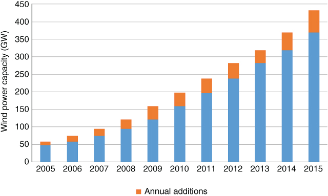
Figure 8.12 Global wind power 2005–2015. Data courtesy of REN21 Global status report 2016.
8.6.1 Theory of Wind Energy
A wind turbine extracts power from the wind by slowing it down. At stand still, the rotor obviously produces no power; at very high rotational speeds, the air is more or less blocked by the rotor, and again no power is produced.
The power produced (![]() ) by the wind turbine is determined from the net kinetic energy change across it (i.e. from the initial air velocity of
) by the wind turbine is determined from the net kinetic energy change across it (i.e. from the initial air velocity of ![]() at inlet to a turbine exit air velocity of
at inlet to a turbine exit air velocity of ![]() , see Figure 8.13) and is described by:
, see Figure 8.13) and is described by:

Figure 8.13 Ideal wind energy theory.
The mass flow rate of wind is given by the continuity equation as the product of density, area swept by the turbine rotor and the approach air velocity:
Hence, the power becomes:
where ![]() is the average speed between inlet and outlet:
is the average speed between inlet and outlet:
Substituting, the power becomes:
To find the maximum power extracted by the rotor, differentiate Equation (8.9) with respect to ![]() and equate it to zero:
and equate it to zero:
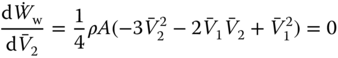
Since the area of the rotor (A) and the density of the air (ρ) cannot be zero, the expression in the bracket has to be zero. Hence, factorizing the quadratic equation:
Since ![]() is unrealistic in this situation, there is only one solution:
is unrealistic in this situation, there is only one solution:
Substitution of Equation (8.11) into Equation (8.8) results in:
Equation (8.12) clearly shows that the power:
- Is proportional to the density (ρ) of the air, which varies slightly with altitude and temperature.
- Is proportional to the area (A) swept by the blades and thus to the square of the radius (R) of the rotor.
- Varies with the cube of the wind speed
 . This means that the power increases eightfold if the wind speed is doubled. Hence, one has to pay particular attention with respect to site selection.
The value in brackets in Equation (8.12) (0.5925) is termed the Betz limit and indicates the theoretical maximum fraction of the power in the wind that could be extracted by an ideal wind turbine. Maximum efficiency depends on optimal wind velocity ratio conditions.
Away from optimal conditions, the theoretical output of the wind rotor is adjusted by the application of a power coefficient, Cp. The variation in power coefficient with wind velocity ratio is shown in Figure 8.14.

Figure 8.14 Variation in power coefficient with velocity ratio.
8.6.1.1 Actual Power Output of the Turbine
Equation (8.12) does not take into account the mechanical and electrical losses incurred in the production of electricity from a wind turbine. Allowing for non‐optimal aerodynamic conditions and gearbox/electrical generator efficiencies (![]() and
and ![]() ), the following can be used to predict the shaft power of a wind rotor:
), the following can be used to predict the shaft power of a wind rotor:
The effect of these factors can be examined by considering the world's largest wind turbine generator which has a rotor blade diameter of 126 metres (rotor swept area 12 470 m2) and is located offshore at sea level where the air density is approximately 1.2 kg/m3.
At its rated wind speed of 14 m/s, the theoretical wind power produced is given by Equation (8.12) and is approximately 12 MW. However, the turbine is rated at 5 MW.
The difference in values indicates the influence of the power coefficient Cp and inefficiencies in the electrical and mechanical power transmission.
Care must be taken when selecting a turbine and assessing the likely energy generation, as the ‘rated power’ is only available when the wind turbine speed reaches a certain level, known as the rated speed. Wind turbine speed performance is split into four different stages:
- Start‐up speed – The speed at which the rotor and blade assembly begin to rotate.
- Cut‐in speed – The minimum wind speed at which the wind turbine will generate any usable power. This wind speed is typically between 3 and 4.5 m/s for most turbines.
- Rated speed – The minimum wind speed at which the wind turbine will generate its designated rated power.
- Cut‐out speed – The wind speed at which the turbine is intentionally shut down. This is a safety feature to protect the wind turbine from damage. It is facilitated using an automatic brake or ‘spoilers’, which are drag flaps mounted on the blades or the hub, activated by excessive rotor revolutions. Alternatively, the entire machine may be turned sideways to the wind stream at high wind speeds.
8.6.2 Wind Turbine Types and Components
There are two types of wind turbine, distinguished by the axis of rotation of the rotor shafts:
- Horizontal‐axis wind turbines, also known as HAWT types, have a horizontal rotor shaft and an electrical generator, both of which are located at the top of a tower. The gearbox/generator housing is termed the nacelle.
- Vertical‐axis wind turbines (VAWT types) are designed with a vertical rotor shaft and a generator and gearbox placed at the base of the turbine. The turbine has a uniquely shaped rotor blade that is orientated to harvest the power of the wind no matter in which direction it is blowing.
Examples are shown in Figure 8.15.

Figure 8.15 Wind turbine types – vertical and horizontal axis.
8.7 Hydropower
Hydropower is power derived from the force of moving water. Hydropower is a versatile, flexible technology that, at its smallest, can power a single home and, at its largest, can supply industry and the public with renewable electricity on a national and even inter‐regional scale.
Hydropower is pollution‐free, has a fast response time and can provide essential back‐up power during major electricity outages or disruptions. Hydropower plants also provide a potential flood‐control mechanism, extracting excess water from rivers. Finally, as part of a multipurpose scheme, impoundment hydropower creates reservoirs that offer a variety of recreational opportunities, notably fishing and water sports.
Hydropower is the largest source of renewable energy generation worldwide. In 2015, the total global capacity was 1064 GW, with a generation of 3940 TWh (REN21, 2016).
Global installed hydropower capacity was in the region of 1000 GW in 2010 and the trend remains upwards. The world leaders in hydropower are China, Brazil, Canada, the United States and Russia. Together these countries account for 52% of total installed capacity. Norway's electricity‐generation system is almost 100% hydro, and there are a number of countries in Africa that produce close to 100% of their grid‐based electricity from hydro (see Figure 8.16).

Figure 8.16 World capacity of hydropower. Data courtesy of EIA, international energy statistics.
8.7.1 Types of Hydraulic Power Plant
There are two types of hydropower plant in use: run‐of‐river schemes and storage systems.
8.7.1.1 Run‐of‐river Hydropower
Run‐of river hydropower schemes (see Figure 8.17) require a bifurcation or separation of a proportion of the flow via a weir impoundment system (1).

Figure 8.17 Run‐of‐river system characteristics.
The take‐off canal (2) is commonly called the headrace or leat.
At the end of the headrace is a settling tank (3), often called the forebay.
The forebay/headrace may contain spillways (4) to return excess flow to the river. From the forebay, the water enters a pipe (5), commonly called the penstock, to commence the final leg of its journey down to the hydro‐turbine. If a site has difficult topography or is environmentally sensitive, the canal is sometimes omitted and an extended penstock carries water from the river bifurcation direct to the powerhouse.
The hydro‐turbine and electrical generator are sited in the powerhouse (6).
After passage through the turbine, the water is returned to the river or stream via a calming channel (7), known as the tailrace.
In a barrage scheme arrangement, the headrace and penstock are dispensed with and the powerhouse is effectively in‐line with the river or stream.
Whether considering an impoundment or a barrage scheme, the fraction of flow diverted for energy generation must not leave the depleted region (reach) of the river ecologically damaged, and consequently, extensive local hydrological and biological studies are carried out prior to scheme sizing.
8.7.1.2 Storage Hydropower
Typically, these are large systems that use a dam to store water in a reservoir (see Figure 8.18). Electricity is produced by releasing water from the reservoir through a turbine, which activates a generator.

Figure 8.18 Typical storage hydropower plant.
Storage hydropower provides base load as well as the ability to be shut ‐down and started up at short notice according to the demands of the system (peak load). It can offer enough storage capacity to operate independently of the natural hydrological inflow for many weeks or even months.
8.7.2 Estimation of Hydropower
In a storage hydropower system, the amount of power produced from water is proportional to the potential energy available, due to the difference of head between the surface levels of the upper and lower reservoirs and the mass flow rate of water going through the turbine.
For a reservoir head difference of h (m), the general equation for fluid power ![]() (W) is:
(W) is:
However, the actual power produced by the turbine unit is less than is indicated by Equation (8.14) because of frictional losses (Δhf, m) in the transmission pipework and the turbine's efficiency (ηt, %). If the efficiency of the electrical generator is (ηgen, %), the power output (![]() ) of the system is:
) of the system is:
Run‐of‐river schemes are also evaluated in terms of flow rate (m3/s) and head difference or river fall (m).
8.7.3 Types of Hydraulic Turbine
Traditionally, there are three different types of turbine used in hydropower generation: the Pelton wheel, the Francis turbine and the Kaplan turbine, each of which has different characteristics to suit the available head (m) and discharge or flow rate (m3/s) (see Figure 8.19).

Figure 8.19 Typical hydraulic turbine specifications.
For low‐head, run‐of‐river schemes, technology with a long history is being employed – the Archimedean screw. This technology was first used over 2000 years ago as a pump for lifting water from a river to its bank. However, in power‐generation schemes, a portion of the flow is diverted and the head variation or fall along the river (perhaps via a weir) is used to drive the screw. The screw shaft is connected to a generator, as shown in Figure 8.20.

Figure 8.20 Archimedean screw turbine.
8.8 Wave and Tidal (or Marine) Power
Large‐scale water waves on the earth's surface are largely caused by the gravitational pull of the moon (the tides) and underwater earthquakes (‘tsunami’). Smaller‐scale water surface disturbances or waves are generally caused by the wind blowing across a water surface. Wind‐generated waves have the potential for energy extraction because water has been ‘lifted up’ from its undisturbed level and given a circular motion. The motion, i.e. the kinetic energy available, extends below the water surface but decreases with increasing depth.
8.8.1 Characteristics of Waves
The motions of real water waves are complex. Simple analyses assume they have a regular repeating pattern of crests and troughs, as shown in Figure 8.21.

Figure 8.21 Wave variables.
The distance between any two repeating points on the wave is called the wavelength (metres). The time taken for a wave to travel a distance of 1 wavelength, that is to complete a cycle, is called the period (T, seconds). Typical values of ocean wave periods are in the range 1–30 seconds. Storm and earthquake waves can have periods ranging from minutes to hours.
This factor is important, as the power (watts) available in a water wave increases directly with period, so, for example, a wave with a period of 10 seconds will, potentially, have two times more power than a wave with a period of 5 seconds.
The maximum vertical disturbance distance from wave crest to wave trough is called the wave height (H, metres) and depends on the prevailing wind regime.
The term amplitude (a, metres) is used to describe ½ the wave height.
This factor is important, as the power (watts) available in a water wave increases with the square of the amplitude, so, for example, a wave with an amplitude of 2 m will, potentially, have four times more power than a wave with an amplitude of 1 m.
8.8.2 Estimation of Wave Energy
The energy per metre of wave crest and unit of surface is given as:

where ρ (kg/m3) is the density of water.
It can be shown that the wave power available is given by:

8.8.3 Types of Wave Power Device
There are several varieties of wave energy converter (WEC).
If deep water is available close to the shoreline, waves may be directed up a focusing ramp arrangement over a sea wall into a collection tank or reservoir in a so‐called wave capture system. At the base of the reservoir is a low‐head water turbine through which water is returned to the sea.
Essentially, this arrangement is recreating a typical hydroelectric scheme with seawater (see Figure 8.22).

Figure 8.22 Wave power device – wave capture absorber.
In oscillating‐column devices, the up and down motion of the water wave is used to create a mirrored motion in a volume of enclosed air (see Figure 8.23). The air can only exit its enclosure by passing through an air turbine connected to an electrical generator. The air direction will, of course, change as the water wave rises and falls, but this is overcome by use of a machine called a Wells turbine whose rotational direction is insensitive to the flow direction of the air. Shoreline and floating varieties of this kind of device have been demonstrated to have potential for significant energy generation.

Figure 8.23 Wave power device – oscillating‐column absorber.
Point absorber wave energy devices usually employ a float to utilize the reciprocating aspect of a wave. Energy conversion and take‐off can take a range of forms, as shown in Figure 8.24. For example, the resulting motion can be used to drive a simple hydraulic pump to transfer a fluid to a reservoir and generator set.

Figure 8.24 Wave power device – floating point absorber.
Alternatively, the reciprocating motion can be used directly to drive a permanent magnet linear generator (a set of coils and magnet stack) mounted on the seabed.
These devices have the advantage of being insensitive to wave direction (see Figure 8.24).
Point absorbers may also be completely submerged static‐pressure devices. In this case, as a wave with its peaks and troughs passes above the device, a gas‐filled chamber, tethered to the seabed, will experience changes in pressure (due to the height of water above it), which cause it to move up and down relative to a fixed power take‐off point (see Figure 8.25). Again, the motion can be used to drive a pumping system or to generate electricity directly. This arrangement has the advantage of not exposing the system to the most damaging aspects of oceanic existence in the wave zone.

Figure 8.25 Wave power device – static‐pressure point absorber.
Floating and semi‐submerged wave profile or line absorber devices typically rock back and forth and side to side in response to incident waves, i.e. they ride the waves instead of responding solely to the vertical motion. They often comprise replicated, articulated units (see Figure 8.26). The motion experienced at the universal joints is transferred to hydraulic rams that create pressure in a hydraulic system connected to electrical generators.

Figure 8.26 Wave power device – wave‐profile‐following device.
Wave surge devices comprise hinged‐flap structures that oscillate back and forth in a horizontal plane (like a pendulum) with the passage of a wave (see Figure 8.27). The motion is converted into fluid pressure by, for example, a piston arrangement attached to the flap. The piston motion can be used to pump a fluid to a reservoir and electrical generator set.

Figure 8.27 Wave power device – wave surge system.
8.8.4 Tidal Power
The moon and earth are locked together, with a mutual force of gravitational attraction keeping them wedded. The effect is complicated by the planet's oceans, since the liquid and solid parts of the planet feel the pull of the moon to a different extent. The oceans feel it more and, in fact, bulge out towards it in its orbit (and a second bulge is generated on the other side of the planet). This effect is further enhanced, but to a lesser extent, by the proximity of the sun.
As the earth rotates under the bulges, the oceans ebb and flow at the coastline. These are the tides. The difference in height between the highest and lowest level of the tide is termed the tidal range. Out in the deep ocean, the height of the swelling is of the order of 1 m; however, at the ocean's edge, the reducing depth and shape of the coastline can modify the phenomenon, producing much larger tidal ranges. The greatest tidal range in the world is found in the Bay of Fundy (∼ 16 m) in Canada. The second highest tidal range (∼ 15 m) is found in the Severn estuary in the UK.
The time between bulges crossing a point on the planet is approximately 12 hours 25 minutes and is entirely predictable, unlike other forms of renewable energy like wind and solar, making this source very attractive from a power supply management point of view.
This effect can be harvested in two different ways.
8.8.4.1 Tidal Barrage Energy
In tidal barrage schemes, a sea dam is constructed between two adjacent points on a coastline, for example, an estuary, forming a man‐made basin. The basin water volume and difference between water levels across the dam can be controlled via sluice gates. The dam also contains a series of turbo‐generators, making this arrangement, in essence, very similar to a hydroelectric system, in that the energy is produced as a result of a difference in head (h) across the turbine. At its simplest, the greater the tidal range, the greater the potential for energy production. With the utilization of turbines that are insensitive to flow direction, the sluice/turbine arrangement has a good degree of flexibility for ebb/flow generation and/or making the basin available for storage considerations.
Depending on maritime traffic, barrage schemes may require a navigation lock. However, barrages can also double as bridges, providing new road links across the chosen estuaries.
The general characteristics of a tidal barrage scheme are shown in Figure 8.28.

Figure 8.28 General characteristics of a tidal barrage scheme.
The average fluid power generated by a scheme can be estimated from Equation (8.14), i.e. ![]() .
.
In the case of a tidal scheme, the basin volume is the product of basin area (A) and the tidal range (h). The tidal flow rate will be the basin volume divided by the time between tides, i.e. 4.47 × 10⁴ seconds.
Finally, the power is calculated using the tidal range mid‐point (h/2) thus:

8.8.4.2 Tidal Stream Energy
These systems take advantage of the high‐speed ocean flows that can occur between islands or between an island and a coastline. The energy‐collection devices often sit on the seabed and resemble submerged wind turbines.
8.9 Thermoelectric Energy
Energy harvesting is a term commonly applied to the scavenging of a previously untapped small‐scale ambient source of energy. Sources of energy for harvesting include light, thermal gradients, vibration and radio frequency radiation. The scale of collection is typically from microwatts to milliwatts. There are many potential demands for this power level, with applications including condition monitoring in construction, health and general manufacture. Energy scavenged from ambient sources may be able to recharge or even eliminate the requirement for a battery in some mobile applications.
Research in this area is being conducted in parallel with energy storage devices (e.g. rechargeable batteries or supercapacitors) and efficient power management circuits to provide a stable power source.
There are many energy‐harvesting conversion technologies available. Here, the direct conversion of thermal energy to electricity and thermoelectric generators will be considered.
8.9.1 Direct Thermal Energy to Electrical Energy Conversion
The discovery of direct thermal to electrical energy conversion is not recent. In early‐1830s Berlin, Thomas Johann Seebeck heated the junction of a circuit comprising two different metals. He detected a magnetic field close to the circuit but failed to make the link with the presence of a voltage in the circuit. Nevertheless, his work is celebrated by the term Seebeck effect.
Consider the open circuit in Figure 8.29 comprising two different material electrical conductors forming a junction. With a suitable electron intensity difference between the two materials at the heated junction, the application of a little heat input is sufficient to allow electron flow, realizing a potential difference detectable across the circuit.

Figure 8.29 Seebeck effect.
The magnitude of the voltage is proportional to the temperature of the junction and the chosen materials.
The slope of the voltage–junction temperature relationship is termed the Seebeck coefficient (αab, V/K) for the combination of materials a and b.
Mathematically:

where ![]() .
.
The absolute Seebeck coefficient of an individual material (αi) can be determined by connecting it in a circuit with a superconductor. A comparison of some material Seebeck coefficients at 100 °C is shown in Table 8.3.
Table 8.3 Seebeck effects for some common materials.
| Material | Seebeck coefficient (α, V/K) |
| Silicon | −455 × 10−6 |
| Constantan | −47 × 10−6 |
| Platinum | −5.2 × 10⁻⁶ |
| Aluminium | −0.2 × 10⁻⁶ |
| Copper | +3.5 × 10⁻⁶ |
| Iron | +13.6 × 10⁻⁶ |
| Germanium | +375 × 10−6 |
Notice that some material coefficients are quoted as positive and some negative. This convention is determined by the resulting flow direction in the circuit.
In 1834, French physicist Jean Peltier applied an electric current to a circuit comprising two dissimilar metals. He discovered that one of the circuit junctions increased in temperature while the other was cooled. He also found that the temperature change depended on the magnitude of the current and that if the current flow was reversed, the junction conditions reversed.
Consider the circuit in Figure 8.30 comprising two different material electrical conductors forming two junctions and a voltage source.

Figure 8.30 Peltier circuit.
With a current flowing in the circuit, it is found that heat is absorbed at one of the junctions (cold junction) and released at the other (hot junction).
The magnitude of the effect is expressed by the Peltier coefficient (πab, volts), which is a function of current (I) and is defined thus:

where Q is the heating (or cooling) effect.
This is essentially a phenomenon coupled with the Seebeck effect and the two are linked by:
where T is the absolute junction temperature in Kelvin.
8.9.2 Thermoelectric Generators (TEGs)
In energy‐harvesting terms, a Peltier device consists of a circuit comprising two dissimilar materials, two junctions, a heat source, a heat sink and a connected external load. A current can be generated in the bi‐material circuit when one junction is heated and the other cooled.
Potentially (p and n type) semiconductors make better thermoelectric generators than metals because of their higher Seebeck coefficients.
A schematic of a semiconductor, single junction thermoelectric generator is shown in Figure 8.31.

Figure 8.31 Thermoelectric generator.
For useful power production, such units are usually connected in a series/parallel arrangement where a number of p‐type and n‐type semiconductor materials are sandwiched between electrically insulated ceramic plates joined together by interconnected copper pads.
The power generated in the thermoelectric circuit ![]() is given by:
is given by:
From Ohm's Law and the Seebeck voltage–temperature relationship:

The resistance of the generator is given by:
where A (m2) is the cross‐sectional area of the TEG circuit, L (m) its length and ρ its resistivity (Ω/m).
Substituting into the above, the total power generated by a thermoelectric device is given by:

The thermoelectric generator will be connected in series with the external load. The power expended at an external load will depend on its resistance and resulting current.
For the device described, the efficiency will be the power available across a connected load divided by the power input to the hot junction or heat source.
In general, efficiency values for thermoelectric generators tend to be low, with values below 10% being commonly reported.
However, they have no moving parts, are compact and can use almost any source of thermal energy as the hot source.
8.10 Fuel Cells
Chemical reactions are, to a great extent, concerned with the rearrangement of electrons between chemical species. In a combustion reaction between hydrogen and oxygen, this results in a great deal of thermal energy being released that can be used to generate electricity by heating up a working fluid and using it to drive some kind of prime mover like a steam or gas turbine at low efficiency.
In a fuel cell, the electron exchange between the hydrogen and oxygen contributes directly to the generation of an electrical current without the need for any intermediate stages.
At a basic level, the components of a fuel cell are similar to those of a battery: anode, cathode, electrolyte and external circuit.
However, unlike a battery, in a fuel cell, complete discharge cannot occur because the cell is constantly supplied with electron donators and acceptors in the form of hydrogen and oxygen. On combination, the reactions produce an electrical current in an external circuit, water and some waste heat. The generic components of a fuel cell are shown in Figure 8.32.

Figure 8.32 Generic fuel cell.
8.10.1 Principles of Simple Fuel Cell Operation
- At the anode, hydrogen undergoes a catalytic reaction, splitting into ions (2H+) and electrons (2e−).
- Ions traverse the electrolyte; electrons flow through the external circuit.
- At the cathode, hydrogen ions, oxygen and electrons from the external circuit form water in a catalyst‐assisted reaction.
A simple arrangement such as this might generate up to 1 volt DC.
Practical fuel cells comprise repeating units of the above in series, forming a stack to produce a more useful level of power. The number of repeating units determines the voltage and the ionic transfer (or transverse) area determines the current.
Electronic conditioning is required to produce AC power with grid‐compatible parameters.
With hydrogen as the fuel, the technology is carbon‐free at the point of generation. Questions remain over the source of hydrogen for use in such cells. Current potential sources include separation from hydrocarbons (e.g. methane can be reformed into H2 and CO2) or the splitting of water. Both are potentially energy‐intensive.
8.10.2 Fuel Cell Efficiency
Care must be taken when quoting the efficiency of a fuel cell. In thermodynamic terms, the reversible cell reaction efficiency (ηreaction) is defined by considerations of molar gas flows (![]() , moles), Gibbs energies (
, moles), Gibbs energies (![]() , kJ/mol) and enthalpies (
, kJ/mol) and enthalpies (![]() , kJ/mol) at a given temperature and pressure:
, kJ/mol) at a given temperature and pressure:

This provides an estimate of the maximum efficiency attained in the absence of irreversibilities. The equation is often quoted in terms of the molar‐based higher heating value (HHV) of the fuel thus:

At room temperatures and pressures, ![]() and
and ![]() .
.
Therefore, for a pure hydrogen–oxygen fuel cell operating at standard temperature and pressure, this equation returns an impressive 83% efficiency. The reaction efficiency decreases with increasing temperature. At 1000 °C, the reaction efficiency drops to around 65%.
This is not the full story, however. Fuel cells rely on physical and chemical processes, for example, reaction and concentration kinetics, mixing, migration, absorption and dissolution, for their operation. These are neither instantaneous nor perfect.
From work considerations, the reversible electrical potential (E, volts) of the fuel cell is given by:

where ![]() is the number of kilomoles of valence electrons flowing in the external circuit and F is Faraday's constant (96.487 kJ/kmol V). For hydrogen,
is the number of kilomoles of valence electrons flowing in the external circuit and F is Faraday's constant (96.487 kJ/kmol V). For hydrogen, ![]() .
.
The voltage efficiency (ηvoltage) of the fuel cell is expressed as the ratio of the actual voltage (V) appearing across the cell compared to the theoretical potential:
The voltage efficiency is inversely proportional to the load current.
Furthermore, an amount of fuel in excess of stoichiometric is usually supplied to the cell to compensate for poor fuel usage, and a third term, the fuel utilization efficiency (ηfuel), is used to describe its impact. It is expressed as the reciprocal of the ratio of actual fuel input (nfuel,act) divided by the stoichiometric amount of fuel (nfuel,act/nfuel,sto). Then:

8.10.3 Fuel Cell Types
The specifications of some of the more common fuel types are detailed in Table 8.4. The cell names usually reflect the electrolyte used. In all cases, the fuel is assumed to be hydrogen.
Table 8.4 Types of fuel cell. Adapted from Hodge, B.K. (2010) Alternative Energy Systems and Applications, John Wiley & Sons, Inc.
| Cell type | Ion carrier | Oxidant | Catalyst | Electrolyte | Operating temperature (°C) | Capacity (MW) | Efficiency (%) |
| Alkaline (AFC) | OH− | O2 | Platinum/palladium | Aqueous potassium hydroxide | Up to 250 | Up to 0.01 | 50–60 |
| Phosphoric acid (PAFC) | H+ | Air | Finely dispersed platinum | Liquid phosphoric acid in silicon carbide matrix | ∼ 200 | 0.01–0.4 | 35–45 |
| Molten carbonate (MCFC) | CO23− | O2 | Nickel/nickel oxide | Molten lithium carbonate/potassium carbonate in porous ceramic matrix | Up to 650 | 0.025–10 | 50–60 |
| Solid oxide (SOFC) | O2− | Air | Non‐precious metals | Solid ceramic, e.g. zirconium oxide | Up to 1000 | Up to 10 | 50–60 |
| Proton or polymer exchange membrane (PEMFC) | H+ | Air | Platinum/ruthenium coating | Acid in thin plastic polymer membrane | Up to 90 | Up to 0.025 | 40–50 |
8.11 Energy Storage Technologies
Our electrical energy demand varies by month, by day, by hour and even by minute. This is a problem for power suppliers because, for reasons of stability, fossil fuel and nuclear power plants are not, in general, able easily to mirror a rapidly varying demand. Moreover, generating capacity must be available to cover the peak demand that may only occur for a small fraction of the day. Some of the criticisms aimed at renewable electrical energy forms are that they are unreliable, unpredictable (with the exception of tidal power) and exacerbate the problem of supply–demand matching. One solution being proposed is the construction of pan‐continental super‐grids, allowing surplus power capacity in one region of a continent to be routed to another experiencing its peak demand. Another potential solution is to generate electrical energy whenever available and store it until demanded.
8.11.1 Energy Storage Characteristics
The salient operating parameters when considering which form of energy store to employ are:
- Energy density (J/m3) – the energy stored per unit volume of store.
- Specific energy content (J/kg) – the energy stored per unit mass of store.
- Storage efficiency (%) – the fraction of the input energy that is usefully recovered.
- Retrieval rate and depletion time (W, hrs) – how quickly and for how long the energy exchange can be maintained.
- Capital and operating costs (£).
8.11.2 Energy Storage Technologies
There are a number of storage technologies which may suit a particular application. Final selection should be based on the criteria previously described.
8.11.2.1 Hydraulic Energy
Electrical energy can be stored by using it to increase the potential energy of water in a pumped storage scheme (see Figure 8.33). This requires a mountainous terrain, as excess electricity is used to pump water from a low‐level lake or reservoir to another lake or reservoir at high elevation. At times of increased electricity demand, water is run back down to the lower reservoir via a turbine connected to an electrical generator. The pumping and generating functions are usually combined into one hydraulic machine (i.e. a pump/turbine).

Figure 8.33 Pump storage scheme.
The specific energy content is approximately 10 J/kg per metre elevation.
Potential energy, i.e. the energy associated with a mass (m) at a vertical distance (h, metres) above ground level in the earth's gravitational force field, is given by:
Typical efficiencies are around 80%, with outputs in excess of 100 MW being brought on line and up to full power in seconds. Output can be maintained for hours, making the technology very useful for supply management purposes and smoothing out variations in renewable energy grid input.
The deployment of these systems is facilitated by using surplus energy from the grid at times of low power demand (usually at night) and cheap‐tariff electricity.
The ratio of energy supplied to the network and the energy consumed during the pumping cycle must be considered to evaluate the overall viability of the scheme.
8.11.2.2 Pneumatic Energy
Energy can be stored by forcing the molecules of a gas into close proximity with each other, i.e. by compressing the gas and increasing its density in a compressed‐air energy storage scheme (CAES).
When the pressure of the gas (typically 50–70 bar at 50 °C) is later reduced, the molecules will spring apart, releasing the stored energy.
In practical terms, excess electrical energy is used to compress air by forcing it into a closed pressure vessel. Large‐scale pressure vessels are very expensive, and so natural cavities, like disused salt mines, have been used as containers. When electrical demand increases, the compressed air is released to a turbine generating electricity (see Figure 8.34).

Figure 8.34 CAES scheme.
If the compression is carried out isothermally, the energy of compression is given by:

where P2 is the storage pressure and V2 the storage volume.
Expanding the air directly during generation will result in a large temperature reduction. In order to protect the turbine, natural gas is used to reheat the air. Alternatively, the heat of compression may be used for this function if a thermal store is provided to operate in parallel with the pneumatic store.
Power outputs are of the order of 1–100's MW, with energy‐depletion times in hours. Care must be taken with definitions of efficiency to include air cooling, drying, reheating of the air etc. Recent developments include cooling the air to its liquefaction point to reduce storage volume.
Again, the technology is very suitable for supply management.
8.11.2.3 Ionic Energy
On a small scale, electrical energy can be stored in rechargeable (or secondary) batteries.
Here, excess electrical energy is converted to electrochemical energy during charging and the reverse during discharge. Performance depends on the rate of charge/discharge.
Lead–acid batteries (specific energy content ∼ 0.14 MJ/kg) have been used for many years for applications of < 10 MW and depletion times of around an hour.
Other materials are available, like nickel–iron and nickel–cadmium (specific energy content ∼ 0.09 MJ/kg). Silica oxide‐based batteries have energy storage capacities of up to 0.4 MJ/kg.
Newer systems like flow (pumped electrolyte) batteries (specific energy content ∼ 1–3 MJ/kg) have better performance, and, with power outputs in the Megawatt range and energy depletion times of up to 10 hours, are being considered for supply management and renewable energy smoothing (see Figure 8.35).

Figure 8.35 Flow battery schematic.
8.11.2.4 Rotational Energy
Electrical energy can be stored by converting it to rotational kinetic energy in a flywheel. The amount of energy that can be stored depends on the mass of the flywheel, the square of its radius and the square of its rotational speed. So, a small change in speed will produce better returns than a small increase in mass. The kinetic energy associated with rotational motion (Wrotate, Joules) about an axis can be evaluated from:
where Im is the moment of inertia (kgm2) that depends on the dimensions (radius, r; mass, m) and the position of the axis of rotation of the body in the relationship:
The factor k for some simple geometries is given in Table 8.5.
Table 8.5 Geometric k factors.
| Geometric shape | k |
| Rim‐loaded thin ring | 1 |
| Uniform disc | 1/2 |
| Thin rectangular rod | 1/2 |
| Sphere | 2/5 |
| Spherical shell | 2/3 |
The angular velocity of the body, ω (rad/s) can be determined with either knowledge of the time taken for one complete revolution of the body, t (seconds) or its rotational speed in revolutions per minute (N), thus:
Typical wheel peripheral speeds are 1500–2000 m/s or rotational speeds of 100 000 rpm. The maximum amount of energy that can be stored depends on the ratio of the strength of the flywheel material and its density. The best type of material would have high strength and low density, so, for example, carbon fibre (specific energy content ∼ 0.77 MJ/kg) would make a better flywheel than steel (specific energy content ∼ 0.17 MJ/kg). Storage efficiency (typically in the range 95–98%) is affected by friction losses, so flywheels often operate on magnetic bearings in a vacuum. Power outputs are limited to less than 1 MW and energy‐depletion times are measured in minutes, putting them on the boundary for supply management.
8.11.2.5 Electrostatic Energy
A device capable of storing electrical energy in the form of an electric field is termed a capacitor. A capacitor comprises a material separating two plates capable of accumulating and maintaining an electric charge potential between them.
For a given voltage, V, the energy storage (Wcap, Joules) of a capacitor is given by:
where C (Farad) is the device capacitance.
The capacitance is a characteristic dependent on the material properties and dimensions of the device.
Super‐capacitors and ultra‐capacitors (specific energy content up to 0.03 MJ/kg) are electrical devices that charge much like a battery but discharge electrostatically. Storage efficiencies are high (98%) but power outputs of less than 100 kW are only possible for a few seconds, and so use is confined to maintaining the quality of a power supply.
8.11.2.6 Magnetic Energy
A device capable of storing electrical energy in the form of a magnetic field is termed an inductor. An inductor can be as simple as a current‐carrying coil of wire.
For a given current, I (amps) the energy storage (Wind, Joules) of an inductor is given by:
where L is the device self‐inductance in Henrys.
For a simple inductor comprising a coil of wire wound around a structure or core, the inductance is dependent on the core dimensions and material as well as the number of turns of wire in the coil.
At very low temperatures (5–20 K), some metals become superconducting, i.e. they have no electrical resistance. Any current passed through a superconductor will produce a magnetic field capable of energy storage. Superconducting magnetic energy storage systems (SMESs) have energy densities of the order of 6.5 MJ/m3. Power outputs in excess of capacitors are possible, but again their energy depletion timeframe is in seconds.
8.12 Worked Examples
8.13 Tutorial Problems
- 8.1
Estimate the thermal energy liberated by 1 kg/s of U‐235 in a nuclear reactor. Assume the fission of a U‐235 atom yields 190 MeV of useful energy and that 85% of the neutrons are effective in the fission. Take Avogadro's number as 6.023 × 10²³ neutrons/g mol, and
 . [Answer: 766 kW]
 - 8.2
On a bright day at a latitude of 52° North, a solar PV cell of dimension 1 m × 1 m will generate a current of 2 A and a voltage of 5 V.
- What power (W) is being generated per cell?
- How many such PV cells are required to generate 1 kW?
- 8.3
A solar thermal collector whose active surface is 2 m by 2 m is exposed to a light intensity of 1000 watts/m2.
- Calculate the potential thermal power (kW) available if the unit is operating at 20% efficiency.
- Water is supplied to the collector at 20 °C. Determine the maximum flow rate (kg/hr) through the collector if the requirement is to provide water at 50 °C.
[Answers: 0.8 kW, 22.86 kg/hour]
- 8.4
A two‐bladed horizontal‐axis wind generator has a rotor diameter of 20 metres.
- Operating at a wind speed of 8.1 metres per second, the rotor extracts 35% of the energy of the wind. If the efficiency of the generator in the power train is 85%, find the electrical power output (kW). Take the density of air to be 1.23 kg/m3.
[Answer: 30.5 kW]
- 8.5
A small‐scale hydropower scheme has a gross head of 125 m at a flow rate of 90 litres per second. If the transmission pipework is designed to limit the head loss to 10% of gross head, using the data below, estimate the electrical power output (MW) for the scheme. Data
- Electrical generator efficiency 85%; turbine efficiency 80%.
[Answer: 67.54 kW]
- 8.6
Determine the possible energy available from ocean swells with a wave height of 4 m and a wave energy period of 10 seconds. Assume that the density of water is 1020 kg/m3.
[Answer: 156 kW/m2]
- 8.7
A waste heat pipe with a contact temperature of 420 °C is used as the heat source for a thermoelectric generator. The TEG has the specification shown below. If the heat sink temperature is 10 °C, determine the potential power generation capacity (W) of the device. Specification
- Length: 20 mm
- Cross‐sectional area: 0.004 m2
- Seebeck coefficient: 0.1 V/K
- Resistivity: 1 Ω/m.
[Answer: 336 W]
- 8.8
Determine the energy storage capacity (MJ) of a flywheel comprising a uniform circular disc of 0.5 m radius and 100 kg weight when rotating at 10 000 rpm. Assume k = 0.5.
[Answer: 6.851 MJ]
- 8.9 A pneumatic energy air store has ambient air compressed isothermally to 60 bar. If the store volume is 200 000 m3, determine the energy stored (MWh). [Answer: 136.4 MWh]
- 8.10
Which one of the following devices has a greater energy storage capacity?
- An inductor with a self‐inductance of 20 µHenrys and a current of 13 A.
- A super‐capacitor with a capacitance of 2 µF and an applied voltage of 2.7 V.