
11
Machine Learning Techniques for Face Authentication System for Security Purposes
Vibhuti Jain, Madhavendra Singh* and Jagannath Jayanti
Guru Gobind Singh Indraprastha University, New Delhi, India
Abstract
The modern world is rapidly revolutionizing the way things work. Everyday actions are being handled electronically. Based on this, a sub-division of application in recognition, specifically face recognition, emerged. Face recognition is a technology capable of verifying the identity of an individual using their face from a digital frame against a database. It has been one of the most captivating and prime research fields in the past few decades. The motivation came from the need of automated recognition and verification. Compared with traditional biometric systems, i.e., fingerprint recognition and iris recognition, face recognition has numerous advantages, not just limited to “no-contact” and “user friendly”. Face recognition is currently being used to make the world smarter and safer. It has future scope to be used in finding missing people, e-commerce, education and many fields. Artificial Intelligence is one of the upcoming and important areas in the field of research and development. It solves various image-related tasks using different algorithms. A number of papers have been published on this subject giving an idea of how accurately and efficiently these techniques identify people. This chapter explores general machine learning algorithms and neural network architectures to identify the identity of an individual, comparing them to see which algorithm works best under certain conditions.
Keywords: Machine learning, deep learning, face recognition, security
11.1 Introduction
In today’s busy world, maintenance of both the security of physical property as well as information is becoming increasingly difficult as well as important. To tackle this concern, researchers came up with a solution of a face recognition system. Face recognition is an important solution to many practical problems (e.g., credit card fraud, IOT attacks by intruders, or security breaches in a company or government building, etc.). In most of these situations criminals used to take advantage by easily making fake or duplicate identities through which they were able to commit crimes using someone else’s identity and escape detection, but with the FRS (face recognition system) these problems can be minimized to an extent. Also, now most of these criminals get caught and are punished under the law.
FRS has rapidly developed in the past few decades, hence now it is used in every sector – from healthcare to agriculture, from industries to law enforcement and many more. And with the advancement in technologies, particularly in the field of Artificial Intelligence and Machine Learning, FRS will get more advanced and secure in the future.
Face recognition – an algorithm which can identify or confirm the identity of a person, thing or any other material by analysing their images. It is widely used for security purposes, law enforcement, etc. There are many factors which make a good recognition system, such as a large database of facial images and a system that can analyze the accuracy and efficiency of the FCR. There are many other factors but the two mentioned above are the most important.
In this chapter it is shown how machine learning and deep learning techniques can be employed to develop a face recognition system, and a comparison is done among different techniques used. The main algorithm used is the Convolutional Neural Network (CNN) which is a deep learning algorithm that takes input as image and does mapping on the important features by assigning different weights/biases to various aspects of the image and hence is able to recognize images.
The following machine learning and deep learning techniques are used in the experiment:
- K-Nearest Neighbors
- Support Vector Machine
- Logistic regression
- Naive Bayes
- Decision tree
- Convolutional Neural Network (CNN)
Since many machine learning and deep learning algorithms are used, a basic introduction regarding each is presented in the following section.
11.2 Face Recognition System (FRS) in Security
Facial recognition systems upgraded biometric security to the next level. They are considered more secure than other security techniques due to their high acceptability and uniqueness, and they involve shorter processing time. Using a face recognition system as a security measure in leading institutions and workplaces ensures that there is absolutely no room for vandalism or human error.
There are many applications of face recognition systems in security. A few of these applications are described below.
- Criminal Identification – Most individuals conceal their identity (cover their faces with mask, scarves, etc.) while committing a criminal offence. Face recognition proved to be a tremendous advantage to law enforcement by helping them to recognize a person merely by scanning a masked face. It can also be used to identify unconscious or dead people at crime scenes.
- Bank Services – Most bank services use passwords exclusively as a security measure, but a major drawback of using only passwords is that they’re based on an individual’s knowledge. Moreover, the more complicated passwords become, the easier people tend to forget them. Even security questions aren’t entirely reliable. A professional could use social engineering to learn sensitive information, ultimately compromising the security of bank accounts. Since a face is undoubtedly connected to its owner, face recognition can be offered as a second factor in authentication along with passwords to present more barriers to defrauders.
- Healthcare – Every year the healthcare sector generates large amounts of sensitive data which is an easy target for cyber thieves. In order to safeguard sensitive data, hospitals are examining the use of face recognition techniques. It is also being used to identify patients and access patient registration and records. It helps to stop patient impersonation (when someone tries to get expensive medical treatment for free). In the midst of the global COVID-19 pandemic this technology has helped in tracking down people who are in quarantine without coming in direct contact with them.
- Tracking Attendance – Using a key-card for security access is simple and pretty generic. However, anyone with access to a code/key-card can misuse it, whereas face identification cannot be forged, i.e., only legitimate individuals can gain access. It has other unquestionable advantages such as it can reduce administrative cost, improve employee productivity, and get real-time data of number of hours employees worked, etc.
11.3 Theory
11.3.1 Neural Networks
A neural network is a system/collection of neurons which is used to recognize patterns in a dataset through a process that mimics the functioning and nature of the human brain’s neural network. For instance, when someone hears something, this is called data and is processed by data processing cells known as neurons in the brain, which recognize what sound it is; a neural network works in a similar manner. These networks are used because of their phenomenal ability to extract meaningful information from complex or imperfect data, which can be used to detect complex patterns that are too complicated to be detected by any other computer techniques or humans. They easily adapt to the changing input data as well so that they can give the best solution to the problem in front of the machine and generate new output easily, according to the updated criteria.
The fundamental unit of computation in the neural network is a neuron, also known as a perceptron. It gets its input from an external source or some other perceptrons and calculates an output value to be passed or the final result. A neural network consists of several perceptrons in many layers. A neural network can have one or more layers and each layer can have one or more neurons. The most basic type of neural network comprises three layers: input unit layer connected to a layer of hidden units, which is further connected to an output unit layer.
- Input Unit – First layer. Raw data is fed into this layer of network from which the neural network has to learn.
- Hidden Unit – Layer between input and output layer. This has a function programmed in it which applies relevant values to input and passes it to the output layer.
- Output Unit – Last Layer. This has the output value or label which the neural network is trying to predict.
There are numerous interconnections between layers. These interconnections extend from each perceptron in the first layer to every single perceptron in the second layer, which are called weights between layers. These weights are assigned on the basis of their correlative importance to other inputs. On arranging vectors of weights corresponding to each input perceptron horizontally, a matrix is formed known as a weight matrix [1]. There’s also a trainable bias value present at each perceptron which is not dependent on input value just to add a bit of adjustability. Now if the weight matrix is multiplied with the input vector and a bias vector is added, intermediate perceptron values are obtained.
In spite of the fact that the neural network is a very complicated configuration, it will be ineffective in solving problems because of non-linearity. Regardless of what weights are used, at the end of the day the change in input values will only result in linear change in the output vector [4]. But in the real world this is undesirable as data has non-linear relationships between input and output variables. This problem is solved by introducing an activation function at the end of each perceptron. It can also be used to decide whether input provided by the perceptron is relevant or not. Some popularly used activation functions are:
- ReLU – Stands for rectified linear units. It takes all real-valued inputs and replaces negative values with zero. F(x) = max(0,x)
- Sigmoid – It takes real value input and squishes it to a range between 0 and 1. This function will pass 0 for very small negative values and 1 for large positive values, it is generally used at the last layer.
- Softmax – It takes a vector of real value score and converts it into values between 0 and 1 whose sum is 1.
- Tanh – It takes real value input and convert its to the range [-1,1]
Neural Network learns by following three steps:
- Forward Propagation – Before the first iteration all weights in the network are randomly assigned only then it moves from input to output layer.
- Error Estimation – At the end of iteration at the output layer, error is calculated by checking the deviation/variation from original output.
- Backward Propagation – After error estimation it passes on these values back through the network to calculate gradients. Then all weights are adjusted/updated with the goal of reducing error at the output layer. This method is also known as Gradient Descent.
11.3.2 Convolutional Neural Network (CNN)
Since the mid-twentieth century, the early days of research in artificial intelligence, researchers and computer scientists have been trying to search for a way to get sense out of the visual data present in this world. Extracting, analyzing and learning patterns out of the visual data manually is very tedious work and also time consuming. However, now things have changed rapidly decade by decade, researchers have made so much advancement in this field of work the above tasks have become less onerous, and large stacks of data become easily maintainable [5]. One of many such areas is computer vision. The main objective of the field of computer vision is to see the world as humans do.
It is a known fact that neural networks are good at complex computations and may seem to be perfect for such aims. But now consider an object detection task; this can also be achieved but a problem arises when the image is of high resolution, i.e., made of large pixels; then the number of parameters increases, making the neural network slow and computationally expensive. For instance, if one processes 32*32*3 image, then they’ll get 3072 parameters but if they get high resolution with 1080*1080*3, then it has approximately 3 million parameters to process that too for a single iteration. For tasks like object detection, image recognition, etc., one won’t use traditional neural networks but a specific type known as convolution neural network.
Convolutional Neural Network (CNN) is a deep learning algorithm which takes input as image and does mapping on the important features by assigning different weights/biases to various aspects of the image and hence is able to distinguish different images. Convolution neural networks process input images as tensors (matrix with additional dimensions) [7]. The image which humans see is different from what the computer sees. For example: a color image of size 720x720, its illustration will be 720x720x3 (Channels = 3 (RGB)). Each pixel has a value from 0 to 255 which represents pixel intensity at that point. Convolutional Neural Network comprises two main components:
- Feature Learning
- Classification
Feature Learning comprises a convolution layer and a pooling layer. It carries out the main part of the network’s computational load. In the convolution layer the restricted part of the input image performs dot product with a filter/kernel (matrix of learnable parameters). Features extracted depend on the type of kernel used. Hence it is very important to choose the correct kernel depending upon the feature required [6]. These are a few types of common filters used in CNN:
- Sharpen
- Edge Detection
- Blur
- Masking
If the image is grayscale then the filter will have small width and height but will have the same depth (h x w x 1) as that of the image. The resultant feature map will depend on three parameters:
- Stride – number of pixels by which filter matrix is moved over input matrix. Larger stride results in smaller feature maps. Given that neighboring pixels are closely related, it makes sense to use stride and reduce output size. It is recommended to use a smaller stride than a big stride as it can lead to high information loss. This happens when big strides are taken. It tends to take two pixels which are further away from each other and less correlated.
- Padding – padding is how many extra pixels should be added to an image to maintain its dimensionality. 1 is mostly used for padding.
- Depth – depth is the number of channels in image.
So, the convolution layer results in a feature map with lesser parameters and the same dimensionality.
The pooling layer solely decreases computational power and prevents overfitting by reducing dimensionality of feature maps keeping crucial information. This layer extracts key features from a limited neighborhood. Pooling doesn’t require any parameter. This layer only modifies height and width of feature map; depth remains unchanged as pooling works individually on each depth slice. In common CNN architectures, pooling is performed with stride 2, 2x2 windows and no padding, whereas convolution is done with padding 3x3 windows, stride 1. Some popularly used pooling methods are:
- Max – Maximum value is taken amongst all values lying in pooling region
- Average – Average value of all values lying in pooling region is taken
- Min – Minimum value is taken amongst all values lying in pooling region
- Sum – Sum of all values in the pooling region is taken.
At the end a matrix is created which has less dimensions and only the chief features of the image.
After obtaining features, the input image is transformed into a suitable form for multi-level fully connected architecture, for classifying fully connected layers are used. A fully connected layer is a simple, feed-forward neural network. The output is flattened and fed to a fully connected layer then back-propagation is applied through iterations of training. Over a sequence of epochs, models can differentiate certain low-level attributes in images. Ultimately, an activation function like sigmoid or softmax is applied, classifying the output. Image recognition and classification are the chief fields of its application. Some other applications are facial recognition and verification, and document digitization. Traditional CNN is not the go-to model for every image-related task. Some network architectures based on CNN are:
- LeNet-5
- AlexNet
- VGG 16
- Inception
- ResNet
- DenseNet
11.3.3 K-Nearest Neighbors (KNN)
KNN is an algorithm inspired from real life. It is one of the simplest, most easily implemented supervised machine learning algorithm (one that learns from labelled data) which is used to find solutions to/for regression and classification problems [3]. As one’s surroundings shape their personality, likewise this algorithm presumes that similar things exist in close proximity due to their similar features/properties. The value of a data point is dependent upon the data points around it. It finds the distance between the given query and those data points. There are various methods to measure distance:
- Euclidean distance (default, most commonly used)
- Manhattan distance
- Minkowski distance
- Cosine distance
- Jaccard distance
Subsequently, a certain number of examples (K) closest to the query are picked. Selecting an appropriate value of K is a crucial part of its implementation; it is recommended to choose a value of K that’s neither too large nor too small. For instance, if someone takes K=1: the model will be too specific to a data instead of being generalized and will tend to be sensitive towards noise. The model may accomplish high accuracy on training data but will give unsatisfactory predictions on previously unseen data. On the other hand, if someone takes K=100: the model will become too generalized and will result in inaccurate predictions on both train and test data. For choosing the right K, a trial and error method is generally used, i.e., trying several values of K and using one that works the best. Then the label of the query is selected with majority voting principle (in case of classification) or by averaging the labels (in case of regression) [8].
KNN’s main drawback is it becomes notably slow on increasing the volume of data or number of independent variables and has no ability to handle missing features of data, making it unsuitable to use in a practical environment (use cases) where classifications/predictions need to be made rapidly and accurately. However, KNN shows supremacy when it comes to:
- Implementation
- Small dataset
- Constantly evolving dataset
- Where training is not required
- Just one hyper-parameter given
It is also known as a lazy learning algorithm as at the time of training all it does is save the complete data on memory and does not perform any computations on that data until scoring, i.e., when someone applies a model on previously unseen points. So for training purposes runtime is as good as it gets and runtime of scoring can be exhaustive, varying linearly with the number of data points. Memory usage of KNN also grows linearly with the number of data points provided for training. The performance of this algorithm can be used as a threshold to define the accuracy that is acceptable, even in the worst case.
11.3.4 Support Vector Machine (SVM)
Support Vector Machine sounds intimidating but is based on a simple idea of creating a line/hyperplane (n-dimensional subspace for an n-dimensional space) to separate the data into classes and maximizing the margin. Margin is the smallest (perpendicular) distance between data point and hyperplane. It is a supervised machine learning algorithm which is used to solve both classification and regression problems. At first approximation a basic hyperplane is created and with addition of new points it moves maximizing the margin. From [2], the study supports the hypothesis from this paper that the SVM approach is able to extract all the relevant information from the training data. Support Vectors are the data points closest to the hyperplane, and if removed would result in altered position of the hyperplane and may result in low accuracy. Core elements contributing to SVM accuracy are:
- Choice of Kernel (Mathematical function to manipulate data)
- Proper Tuning of hyper-parameters.
Choosing a kernel to utilize current features to apply some transformations, creating new features (transforming low dimension input space to high dimension) is known as a kernel trick. Radial Basis and Polynomial Function are the most popular ones used. Now in real-world scenarios finding a linearly separable dataset is nearly impossible. So there is some tolerance given to SVM called soft margin to handle misclassifications as the bigger the tolerance is, the narrower the margin.
A combination of soft margin and kernel tricks are used to deal with real-life scenarios like text classification such as spam detection and category assignment, etc.
11.3.5 Logistic Regression (LR)
Logistic Regression is an elemental and popular algorithm used to solve classification problems. It is a supervised machine learning algorithm; it is named as Regression because its fundamental technique is similar to Linear Regression. Linear Regression assumes a linear relation between input independent variables and output dependent variables, and is highly sensitive to outliers in data resulting in poor outcomes/predictions. Logistic Regression uses a logistic function (sigmoid function, which gives output value between 0 and 1) to overcome this drawback. In logistic regression a probability threshold is determined; if the probability of an element is above the threshold then it is classified in one class or vice versa.
There are three different categories of Logistic Regression:
- Binary: Only two possible outcomes
- Multinomial: three or more categories without ordering
- Ordinal: three or more categories with ordering
For determining binary classification, one tries to find the best fitted line first by Linear Regression; then the predicted value is fed into the sigmoid function for conversion to probability. Maximum likelihood estimation is used for calculation of cost function instead of mean squared error, as if this is used it will result in a non-convex function of parameters with many local minima, making it laborious to find global minimum and minimize the cost value. By default this algorithm is limited to binary-class classification, but a popular workaround can be used for multi-class classification, i.e., by splitting the problem into multiple binary classification problems, another alternate approach involves changing the loss function to cross entropy loss and single output probability to one probability per class. One major drawback is it is difficult to obtain complex relationships as linearly dependent data is rarely found in real-world case scenarios, and can only be used to predict discrete sets. However, it is easy to implement, is efficient, accurate and fast at classifying previously unknown data.
11.3.6 Naive Bayes (NB)
Naïve Bayes is a user-oriented powerful supervised machine learning algorithm which uses a series of probabilistic classifier based on Bayes rule with simple assumptions:
- There is no correlation between features or predictors; i.e., they’re independent of each other.
- The features contribute equally, i.e., all carry the same weightage in classification; no feature is given more importance than others.
Naïve Bayes is a generative model (a model which creates new data instances). It is generally used for General Classification and text analytics. It has many configurations, namely:
- Multinomial Naïve Bayes – Computes likelihood to be count of a random variable.
- Complement Naïve Bayes – Instead of computing probability of a random variable belonging to a particular class, it computes the probability of a random variable belonging to all classes.
- Bernoulli Naïve Bayes – Predicators/features are Boolean (binary) variables, the rest is similar to multinomial Naïve Bayes.
- Out-of-core Naïve Bayes – This classifier handles large-scale classification for which complete dataset might not fit.
- Gaussian Naïve Bayes – This involves predictors (input data mapped to target variable) taking a continuous value like in Gaussian/Normal Distribution.
Firstly, one calculates the probability of each class out of all classes which is known as its class prior probability; similarly, the probability of each predictor out of all predictors which is known predictor prior probability is computed. In the third step one calculates probability of likelihood, i.e., probability of predictor given class. Then in the final step posterior probability, i.e., the probability of the class given predictor, is calculated. Now if a model has many features then it is possible that the resulting probability may become zero because one of the attribute’s values is zero [9]. To solve this problem, someone can increase the value of the feature with zero to a small value so that the required probability doesn’t come out as zero. This correction is known as Laplace correction. Gaussian Naïve Bayes shows dominance when it comes to predicting using a small dataset. It performs effectively on categorical input variables as compared to numerical variables. On the contrary, Bayes is considered a bad estimator sometimes, but despite the strong assumptions and cons, this performs extremely well in many cases and is a computationally inexpensive classifier.
11.3.7 Decision Tree (DT)
Decision trees are non-parametric supervised machine learning algorithms which are used for both regression and classification. Decision trees learn directly from the dataset with the help of if-else decision rules in order to estimate a sine curve. They consist of two elements: branches and nodes.
Some chief terminologies associated to decision trees are:
- Root Node: This node marks the start of the decision tree.
- Decision Node: Where a sub-nodes splits into further nodes.
- Terminal/Leaf Node: Last node of the tree, i.e., predicted/ classified label.
- Sub-Tree/Branch: Subdivision of the entire tree.
Decision tree classifies the example by categorizing it down the tree to some terminal/leaf node, providing the classified label. Each and every node represents a test case for some feature, and each edge down from the node giving potential answers. Its accuracy is greatly determined by its ability to make tactical splits. A decision tree uses numerous algorithms to decide that split such as:
- ID3: Iterative Dichotomiser 3 (Extension of D3)
- C4.5: Successor of ID3
- CART: Classification and Regression Tree
- CHAID: Chi-square Automatic Interaction Detection
- MARS: Multivariate Adaptive Regression Splines
First of all, the root node attribute is chosen based on Attribute Selection Measure (ASM), i.e., if a dataset has N attributes then determining which attribute should be placed at the root/internal nodes. It’s not feasible to just select randomly, as it may result in poor results with low accuracy. So certain metrics are used such as Entropy or Gini Index for categorical and Mean Squared or Residual Error for regression, and different processes, depending on whether the evaluating feature is continuous or discrete. For continuous attribute, average of two consecutive values is used as possible thresholds; for discrete attribute, all possible values are evaluated, leading to N calculated metrics for each variable, resulting in N possible values for each categorical value. This process is repeated until stopping criteria is reached. Now this splitting leads to complex grown trees which are more likely to overfit the data, resulting in low accuracy on previously unseen data. A process called pruning is used to ensure good accuracy and prevent overfitting. It reduces the size of trees by turning some branches into leaf nodes, and discarding the leaf nodes under the primary branch, making the tree simpler by structure. A pruned tree has less sparsity than an unpruned tree. After a decision tree is built, predicting a value/label starts from the root of the tree, comparing the root feature with the record’s feature, and then following the branch corresponding to that value until the terminal/leaf node with predicted value is attained. When compared to other algorithms, this doesn’t require large datasets, normalization and scaling of data, and missing values does not affect the building of a decision tree; then again, a small change in data may cause great change in structure of the tree, causing instability. As the complexity of decision rules is directly proportional to the depth of the tree, decision trees need a good amount of time to train the model as sometimes calculations go far more complex than other algorithms.
11.4 Experimental Methodology
11.4.1 Dataset
For this experiment a custom dataset was made and used. The dataset consisted of six folders representing six different people having 45 images of each individual. Images in these folders are of different sizes and are handpicked such that only the front view of the face is taken. All the images are in RGB format.
11.4.2 Convolutional Neural Network (CNN)
- Preprocessing
As the dataset is small and collected images are of different sizes, it is not suitable for direct input in a neural network. Therefore, they are preprocessed according to needs.
The following steps are taken for preprocessing:
- All the images are first loaded and each image is reshaped into dimensions of 64*64.
- After this, integer labels starting from 0 to 5 are given to string labels of images. And data of each folder is shuffled and divided into training and testing dataset randomly in a ratio of 7:3.
- Then the new dataset is augmented using the ImageDataGenerator class of Keras. Data is augmented in order to improve the model’s performance and increase its accuracy by increasing the ability to generalize. It artificially creates new instances of data from an existing dataset by using transforms such as zoom, flip, shift, etc. By augmenting the dataset, it introduces variations of images to the model. The following parameters were given:
- class_mode = categorical, i.e., 2D array of one-hot encoded labels.
- batch_size = 2
- target_size = (64,64)
- zoom_range = 0.2, i.e., random zoom range
- horizontal_flip = True.
- Lastly, the preprocessed dataset is fed to the neural network.
- Convolutional Neural Network for Image Processing
- To make this architecture, the sequential model API of the Keras library is used.
- Three convolutional 2D layers are made with 64, 128, 64 filters, respectively. After preprocessing, the input size of each image is [64, 64, 3] dimensionally. The Foremost Conv 2D layer comprises 64 filters with [5,5] as dimensions of each filter and uses ReLu as activation function. This layer gives output of dimensions [60, 60, 64]. (Due to 64 filters being used third dimension changes to 64, i.e., adds 64 channels to image.) After this a MaxPool2D layer of dimension [2,2] is added to provide an abstract form (avoiding overfitting) and reduce dimensions of output of the first layer. The resultant dimensions are [30,30,64]. This is passed as input to the third layer which is again a Conv2D layer of 128 filters having [5,5] as dimensions, again using ReLu as activation function. This layer gives output of [26,26,128] dimensions. Now again the MaxPool layer is added of dimensions [2,2] giving output with dimensions [13,13,128]. This is used as input for the last Conv2D layer having 64 filters of [5,5] dimensions and activation function ReLu, giving [9,9,64] as output dimensions. Another MaxPool2D layer of [2,2] dimensions is added. This layer gives output of [4,4,64] dimensions. The neural network architecture and summary can be seen in Figures 11.1 and 11.2 respectively below.
- Now a Flatten layer is added to flatten output to pass it to Dense layers for prediction. After flatten output dimension is 1024. Towards the end of the network there are 2 dense and hidden layers of 256 and 128 neurons, and lastly a 6 neuron softmax layer to calculate probabilities.
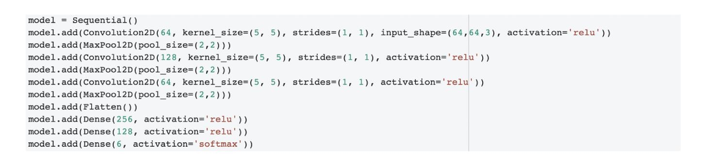
Figure 11.1 Architecture of convolutional neural network.

Figure 11.2 Summary of convolutional neural network.

Figure 11.3 Compilation of convolutional neural network.
- The model is compiled using accuracy as metrics, Adam optimizer and categorical cross entropy because of multiclass classification. The model can be compiled using the program shown in Figure 11.3.
- For predictions: Saved model of “.h5” format is loaded and the “predict” function is called, taking new images as input arguments and making predictions based on them. It gives output as “0” for first individual, “1” for second individual and so on up to 6 individuals.
11.4.3 Other Machine Learning Techniques
- Preprocessing
The number of images collected (dataset) are not suitable to be given to any machine learning technique hence some preprocessing is required.
For preprocessing the following steps are taken:
- All the images are first loaded using the OpenCV module but it loads images in BGR color channel rather than RGB which is required. So in order to obtain an RGB channel, order is reversed.
- Next every image is aligned in the dataset to a particular dimension so that each image is of the exact same dimension from all sides. In this step, other aligned module parameters such as ‘getLargestFaceBoundingBox()’, ‘landmarkIndices’ are also used.
- Now the image is embedded into a vector of zeros, in this image is converted from RGB (255 channels) to an interval between [0,1]. So that the resultant vectorize image contains each pixel with a value of 0,1.
- Now it is necessary to encode the labels for each image. In order to do that a LABEL ENCODER is initialized, which is fitted with the labels from the dataset. At last, the encoder is transformed to a numerical value matrix so that it can be used with a vectorized form of images.
- One final step is taken, to split the images as well as the labels into training and testing data. It is important to shuffle data before splitting.
- K-Nearest Neighbor (KNN)
- First step is to import the “KNeighborsClassifier” from the neighbors model api of the sklearn library.
- This KNeighborsClassifier is used to classify images which is primarily based on the K nearest neighbors (KNN) machine learning technique.
- The classifier has different types of hyperparameters all of which have default values but values can be set on according to requirement.
- In this classifier two hyperparameter are changed:
- n_neighbors = 2 (default : 5)
- metric = ‘euclidean’ (default : ’minkowski’)
- KNN classifier can be initiated as shown in Figure 11.4. Now training data is fitted into the classifier.
- At last the “.predict” function is used to classify the images and with the help of “accuracy score” the accuracy of the classifier is generated.
- Support Vector Machine (SVM)
- First step is to import the “LinearSVC” from the svm model api of the sklearn library.
- This LinearSVC classifier is used to classify images which is primarily based on the Support vector machine (SVM) machine learning technique.
- The classifier has different types of hyperparameters, all of which have default values but values can be set on according to requirement.

Figure 11.4 Summary and Hyperparameters of K-Nearest Neighbor classifier.

Figure 11.5 Summary and Hyperparameters of support vector machine classifier.
- In this classifier three hyperparameter are changed:
- Penalty = ‘l2’
- Loss = ‘squared_hinge’
- max_iter = 1000
- SVM classifier can be initiated as shown in Figure 11.5. Now training data is fitted into the classifier.
- At last the “.predict” function is used to classify the images and with the help of “accuracy score” the accuracy of the classifier is generated.
- Naive Bayes (NB)
- First step is to import the “GaussianNB” from the Naive Bayes model api of the sklearn library.
- This GaussianNB classifier is used to classify images which is primarily based on the Naive Bayes machine learning technique.
- The classifier has different types of hyperparameters all of which have default values but values can be set on according to requirement.
- In this classifier all default hyperparameters are used.
- Gaussian Naive Bayes classifier can be initiated as shown in Figure 11.6. Now training data is fit into the classifier.
- At last the “.predict” function is used to classify the images and with the help of “accuracy score” the accuracy of the classifier is generated.
- Logistic Regression (LR)
- First step is to import the “LogisticRegression” from the linear model api of the sklearn library.
- This Logistic Regression classifier is used to classify images which is primarily based on the Logistic Regression machine learning technique.
- The classifier has different types of hyperparameters, all of which have default values but values can be set on according to requirement.
- In this classifier one hyperparameter is changed:
- multi_class = ‘multinomial’ (default : ‘auto’)

Figure 11.6 Summary and hyperparameters of Naive Bayes classifier.

Figure 11.7 Summary and hyperparameters of Logistic Regression classifier.

Figure 11.8 Summary and hyperparameters of Decision Tree classifier.
- Logistic regression classifier can be initiated as shown in Figure 11.7. Now training data is fitted into the classifier.
- At last the “.predict ” function is used to classify the images and with the help of “accuracy score” the accuracy of the classifier is generated.
- Decision Tree (DT)
- First step is to import the “DecisionTreeClassifier” from the tree model api of the sklearn library.
- This DecisionTreeClassifier is used to classify images which is primarily based on the Decision Tree machine learning technique.
- The classifier has different types of hyperparameters all of which have default values but values can be set on according to requirement.
- In this classifier two hyperparameter are changed according to requirement
- spitter = “best”
- criterion = “gini”
- Decision tree classifier can be initiated as shown in Figure 11.8. Now training data is fitted into the classifier.
- At last the “.predict ” function is used to classify the images and with the help of “accuracy score” the accuracy of the classifier is generated.
11.5 Results
All the classifiers and Convolutional neural network were fitted on the training dataset of images. Training of CNN took a few hours but was able to make precise predictions on input images. It was observed that for a small dataset CNN didn’t perform up to the mark; on the other hand, traditional machine learning algorithms unexpectedly performed well on a small dataset with accuracy ranging from 92% to 97%. If the dataset is skewed (increase number of images belonging to a particular class) it was observed that traditional machine learning algorithms showed highly biased results towards a particular class as compared to convolutional neural networks. Traditional machine learning algorithms and convolutional neural networks show poor results when the input face image provided is not front facing but this restriction will be revoked if convolutional neural network is trained on few images facing other sides. The graph shown below in Figure 11.9, shows the accuracy percentage for each algorithm. Percentage is computed by comparing the number of correctly identified images and total number of tested images.
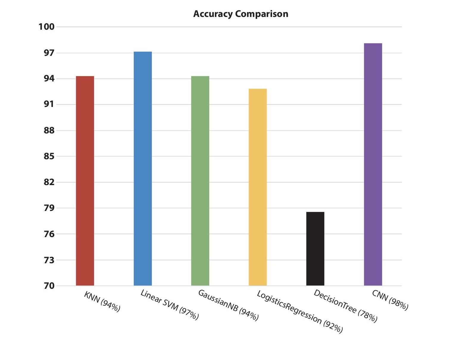
Figure 11.9 Accuracy comparison between convolutional neural network (CNN) and other machine learning techniques.
11.6 Conclusion
Face recognition is one of the most challenging problems in the vast field of computer vision. It has received a lot of attention over the last few decades because of its applications in various sectors [11]. In order to do this a vast amount of research has been conducted over the past few decades, and a lot of progress has been made in this field and results have been encouraging for all the researchers. But a perfect face recognition system that is able to perform adequately under all circumstances and conditions that are applied is still a long way away.
“The human face is a dynamic object and has a high degree of variability in its appearance, which makes face detection a difficult problem in computer vision.”
“Face detection: A survey” [10].
This paper presents an empirical comparison of the different machine learning and deep learning techniques, based on face recognition systems. The results are all satisfactory and promising and they clearly show that CNN (Convolutional neural network) performed better than any other machine learning techniques. But these are only a small set of techniques used while there are many techniques out there which need some research and can perform even better. This gives a future scope in which more prominent and promising techniques can be developed by improving and advancing. There is a need for more advanced research for every methodology so that they can be made for development in various sectors to meet public need. Security and surveillance are the sectors which are most impacted by face recognition systems. Nowadays, there is talk of implementing these face recognition systems in the banking sector (for security, fraud detection, etc.) but still there are some areas where these advanced technologies can be exploited by intruders, hackers, etc., so there is scope for a lot of studies, researches, infrastructure improvement, etc.
References
- 1. Latha, P., Ganesan, L., & Annadurai, S. (2009). Face recognition using neural networks. Signal Processing: An International Journal (SPIJ), 3(5), 153-160.
- 2. Jonsson, K., Kittler, J., Li, Y. P., & Matas, J. (2002). Support vector machines for face authentication. Image and Vision Computing, 20(5-6), 369-375.
- 3. Pandey, I. R., Raj, M., Sah, K. K., Mathew, T., & Padmini, M. S. (2019). Face Recognition Using Machine Learning. IRJET April 2019.
- 4. Serra, X., & Castán, J. (2017). Face recognition using Deep Learning. Catalonia: Polytechnic University of Catalonia, 78.
- 5. Lawrence, S., Giles, C. L., Tsoi, A. C., & Back, A. D. (1997). Face recognition: A convolutional neural-network approach. IEEE Transactions on Neural Networks, 8(1), 98-113.
- 6. Coşkun, M., Uçar, A., Yildirim, Ö., & Demir, Y. (2017, November). Face recognition based on convolutional neural network. In 2017 International Conference on Modern Electrical and Energy Systems (MEES) (pp. 376-379). IEEE.
- 7. Gupta, P., Saxena, N., Sharma, M., & Tripathi, J. (2018). Deep neural network for human face recognition. International Journal of Engineering and Manufacturing (IJEM), 8(1), 63-71.
- 8. Kamencay, P., Zachariasova, M., Hudec, R., Jarina, R., Benco, M., & Hlubik, J. (2013). A novel approach to face recognition using image segmentation based on spca-knn method. Radioengineering, 22(1), 92-99.
- 9. Putranto, E. B., Situmorang, P. A., & Girsang, A. S. (2016, November). Face recognition using eigenface with naive Bayes. In 2016 11th International Conference on Knowledge, Information and Creativity Support Systems (KICSS) (pp. 1-4). IEEE.
- 10. Hjelmås, E., & Low, B. K. (2001). Face detection: A survey. Computer vision and image understanding, 83(3), 236-274.
- 11. Hassaballah, M., & Aly, S. (2015). Face recognition: challenges, achievements and future directions. IET Computer Vision, 9(4), 614-626.
Note
- *Corresponding author: [email protected]