3. Optimal Periodic Software Rejuvenation Policies in Discrete Time

Present-day applications in computer systems impose stringent requirements in terms of software dependability, because system failure, caused by software failure in almost all cases, may lead to a huge economic loss or risk to human life. A guaranteed fulfillment of these requirements is very difficult, especially in applications with nontrivial complexity. In recent years, considerable attention has been paid to continuously running software systems whose performance characteristics are smoothly degrading in time. When a software application executes continuously for a long period of time, some of the faults cause software to age due to the error conditions that accrue with time and/or load. This phenomenon is called software aging and can be observed in many original software systems [1, 2, 3, 4, 5 and 6]. One common experience suggests that most software failures are transient in nature [7]. Since transient failures disappear if the operation is retried later in slightly different context, it is difficult to characterize their root origin. Therefore, the residual software faults are obvious in the operational phase. Grottke and Trivedi [8] classify several software bugs and point out that the resource exhaustion in computer systems causes the software aging. A complementary approach to handle transient software failures is called software rejuvenation [9] which can be regarded as a preventive and proactive solution that is particularly useful for counteracting the phenomenon of software aging. It involves stopping the running software occasionally, cleaning its internal state, and restarting it. Cleaning the internal state of software may involve garbage collection, flushing operating system kernel tables, reinitializing internal data structures, etc. An extreme, but well-known example of rejuvenation is a hardware reboot. In this way, software rejuvenation is becoming much popular as one of the light weighted software fault tolerant techniques.

Huang et al. [9] propose a continuous time Markov chain (CTMC) with four states, that is, initial robust (clean), failure probable, rejuvenation, and failure states. They evaluate both the unavailability and the operating cost in the steady state under a random software rejuvenation schedule. Danjou et al. [10] and Dohi et al. [11, 12, 13, 14 and 15] extend the result of Huang et al. [9] and propose different software rejuvenation models in continuous time, based on a semi-Markov process. Furthermore, Garg et al. [16], Suzuki et al. [17], and Dohi et al. [18] introduce the periodic rejuvenation and develop a Markov regenerative process (MRGP) model to trigger software rejuvenation on computer clock. In the above works, the authors propose nonparametric estimation algorithms with the empirical distribution to estimate the optimal software rejuvenation schedule statistically from the complete sample of failure time data. If a sufficient number of samples of failure time data can be obtained, then the estimates of the optimal software rejuvenation schedules based on Dohi et al.’s algorithm [11, 12, 13 and 14] asymptotically converge to the real optimal solutions. Zhao et al. [19] apply an accelerated life testing technique by injecting memory leaks in their experiments and examine the above nonparametric estimation methods in importance sampling simulation. Rinsaka and Dohi [20] propose another nonparametric estimation algorithm based on the kernel density estimation (see, e.g., Duin [21], Parzen [22], Silverman [23]) to improve the estimation accuracy of the optimal software rejuvenation schedule with a small sample data. Rinsaka and Dohi [24, 25 and 26] use a nonparametric predictive inference (NPI) approach provided by Coolen and Yan [27] and Coolen-Schrijner and Coolen [28]. Though the NPI-based approach is categorized as a prediction-based software rejuvenation, the results obtained by Rinsaka and Dohi [24, 25 and 26] are quite different from those of Vaidyanathan and Trivedi [29] for another prediction-based scheme with linear regression model on system workload.

Apart from the time-based optimal software rejuvenation schedule, some other stochastic models have been proposed in the literature. Bao et al. [30,31], Bobbio et al. [32], Okamura et al. [33], Wang et al. [34], and Xie et al. [35] developed condition-based software rejuvenation schemes, where the system workload is measured to trigger software rejuvenation. Although system parameters and resource usage strongly affect the software aging, it was observed that the mechanism of aging for individual software-based system has to be clarified. In other words, since the aging-related bugs may not be related to system workload explicitly, it may be difficult to apply the workload-based software rejuvenation to tolerate transient failures completely. Pfening et al. [36] formulate a server-type software system with degradation as a queuing system by a Markov decision process. Garg et al. [37] take account of the presence of system failure caused by software aging and analyze the time-based optimal software rejuvenation schedule. This model is extended latter in the study by Okamura et al. [38, 39 and 40] by introducing a different workload-based rejuvenation schedule and/or a more general arrival process of transactions. Recently, Zheng et al. [41] generalized the existing stochastic models [37, 38, 39 and 40] in terms of the rejuvenation policies and arrival stream of transactions. Van Moorsel and Wolter [42] focus on the system restart and derive the optimal restart policies to rejuvenate a software system over finite and infinite operational periods.

It should be worth mentioning that all the above-mentioned software rejuvenation models are formulated under the assumption that the software system operates in continuous time. However, in real-world examples, it is not always possible to monitor and control software systems in continuous time. For example, it is common to back up the system data in file systems at any periodic timing, such as the end of every business hour or weekend. In this sense, the discrete-time models seem to be more realistic to make a decision for software rejuvenation. Dohi et al. [43] and Iwamoto et al. [44] proposed a software availability model and a software cost model operating in a discrete time setting, which are similar to those operating in continuous time [11,12]. Also Iwamoto et al. [45] formulate the discrete-time semi-Markov model under a different criterion called cost-effectiveness which is a mixture of system availability and expected cost in the long run. Iwamoto et al. [46] reformulate the MRGP model in continuous time in [17] and derive the optimal periodic software rejuvenation policy in discrete time by maximizing the steady-state system availability. Unfortunately, the discrete-time models with periodic rejuvenation have not been fully studied yet, so the analysis of expected cost model and cost-effectiveness models also remains incomplete. In this chapter we overview a software rejuvenation scheduling problem and provide a comprehensive survey of the optimal periodic software rejuvenation policies in discrete time under four criteria of optimality: expected cost per unit time in the steady state, steady-state system availability, cost-effectiveness, and expected total discounted cost over an infinite time horizon. The last three criteria are original results of this chapter. We characterize the respective optimal software rejuvenation policies in discrete-time model and provide their associated statistical estimation algorithms from the complete sample of failure time data.

The remaining part of this chapter is organized as follows. In Section 3.2, we describe an MRGP model with periodic software rejuvenation in accordance with Iwamoto et al. [46]. In Section 3.3, we formulate the expected cost per unit time in the steady state and derive the optimal periodic software rejuvenation time minimizing it. We also provide a statistically nonparametric estimator of the optimal periodic software rejuvenation time as a function of system failure time. Sections 3.4 and 3.5 concern the steady-state system availability and cost-effectiveness, respectively. We derive the analytical solutions and nonparametric estimators of the corresponding optimal periodic software rejuvenation policies. In Section 3.6, we consider a somewhat different criterion called the expected total discounted cost over an infinite time horizon. Dohi et al. [13] and Danjou et al. [10] investigate effects on discounting over the expected cost for software rejuvenation models with aperiodic policy [9] and periodic policy [16], respectively. On the other hand, a software cost model with discounting has not been known in discrete time. We formulate the expected total discounted cost over an infinite time horizon and minimize it. Numerical illustrations are given in Section 3.7, where the Monte Carlo simulation is conducted to investigate asymptotic behavior of estimators. Section 3.8 concludes the chapter with some remarks.

3.2 Model Description

3.2.1 Notation

Consider a periodic software rejuvenation model developed by Iwamoto et al. [46]. First, we define the system states and notation as follows:

State 0: highly robust state
State 1: failure probable state
State 2: failure state
State 3: software rejuvenation state
State 4: software rejuvenation state without through failure probable state.

The notation used in this chapter is as follows:

Z: time interval from highly robust state to failure probable state (discrete random variable)

$F_{0} (n), f_{0} (n), μ_{0} (> 0)$ : cumulative distribution function (c.d.f.), probability mass function (p.m.f.), and mean of Z, where n = 0, 1, 2,…

X: failure time from failure probable state (discrete random variable)

$F_{f} (n), f_{f} (n), μ_{f} (> 0)$ : c.d.f., p.m.f., and mean of X

n₀: trigger time of software rejuvenation (integer value)

$F_{a} (n), f_{a} (n), μ_{a} (> 0)$ : c.d.f., p.m.f., and mean of recovery operation time from failure state

$F_{c} (n), f_{c} (n), μ_{c} (> 0)$ : c.d.f., p.m.f., and mean of overhead incurred by software rejuvenation

$c_{s} (> 0)$ : recovery (corrective maintenance) cost per unit time

$c_{p} (> 0)$ : rejuvenation (preventive maintenance) cost per unit time.

3.2.2 Model Description

The system operation of the software system starts at time n = 0 in the highly robust state. For some reason, such that the total amount of memory leaking attains a critical threshold, the process makes a transition to the failure probable state after the time period Z elapses. Just after the state becomes the failure probable state, a system failure may occur with positive probability. If the system failure occurs in the failure probable state before triggering a software rejuvenation, then the corrective recovery operation starts immediately at that time, and is completed after the random time with mean μ_a elapses. Otherwise, the software rejuvenation is triggered as a preventive maintenance of the software system, where the trigger time of software rejuvenation n₀ is measured from the beginning of system operation. This assumption is different from the previous aperiodic model by Dohi et al. [43] and Iwamoto et al. [44,45], because the trigger time of software rejuvenation under aperiodic policies is measured from the time instant when the failure probable state is observed. Of course, this may not be plausible in many cases if the system states (highly robust state and failure probable state) cannot be identified. After completing the recovery operation or software rejuvenation, the system state becomes as good as new, and the software age is initiated at the beginning of the next highly robust state. In the above model, note that the cycle length of software rejuvenation is measured from the time instant just after the system enters State 1 from State 0.

Let us consider the time to trigger software rejuvenation to be a constant integer n₀. We call $n_{0} (\geq 0)$ the software rejuvenation schedule. Define the time interval from the beginning of the system operation to the completion of the preventive or corrective maintenance as one cycle. Figure 3.1 depicts the configuration of our model with periodic rejuvenation. Since the underlying stochastic process is a discrete MRGP with four regeneration states [46], we provide the transition diagram in Figure 3.2, where the states denoted by circles (0, 2, 3, 4) and square (1) are regeneration points and non-regeneration point, respectively, in the MRGP. Strictly speaking, this stochastic process is not a common discrete-time semi-Markov process. However, since only one non-regeneration point is included in the transition diagram, it can be reduced to an equivalent discrete-time semi-Markov process by introducing the convolution of discrete probability distributions [46].

Images

FIGURE 3.1
Configuration of periodic rejuvenation model in discrete time.

Images

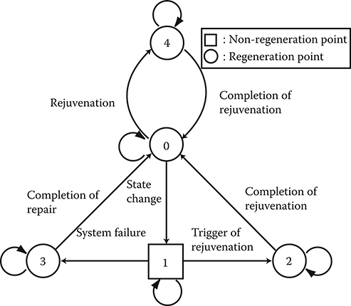
FIGURE 3.2
MRGP transition diagram.

3.3 Expected Cost Analysis

3.3.1 Formulation

In this section, we consider the expected cost per unit time in the steady state. We make the following two assumptions:

Assumption (A-1): $c_{s} > c_{p}$ ,
Assumption (A-2): $μ_{a} > μ_{c}$ .

The assumption (A-1) implies that the recovery cost per unit time is greater than the rejuvenation cost per unit time. On the other hand, in the assumption (A-2), the mean time of recovery operation is greater than the mean rejuvenation overhead. Under these plausible assumptions, the mean time length of one cycle and the expected total cost during one cycle are given by

$\begin{matrix} T (n_{0}) = μ_{a} (F_{f} * F_{0}) (n_{0}) + μ_{c} \bar{(F_{f} * F_{0})} (n_{0}) + \sum_{n = 0}^{n_{0} - 1} \bar{(F_{f} * F_{0})} (n), \end{matrix} (3.1)$

$\begin{matrix} V (n_{0}) = c_{s} μ_{a} (F_{f} * F_{0}) (n_{0}) + c_{p} μ_{c} \bar{(F_{f} * F_{0})} (n_{0}), \end{matrix} (3.2)$

respectively, where $(F_{f} * F_{0}) (n)$ is the discrete Stieltjes convolution of $F_{f} (n)$ and $F_{0} (n)$ , and $\bar{(F_{f} * F_{0})} (n) = 1 - (F_{f} * F_{0}) (n)$ in general. Hence, the expected cost per unit time in the steady state is, from the renewal reward argument, given by

$\begin{matrix} C (n_{0}) = \lim_{n \to \infty} \frac{E [cost occured for [0, n)]}{n} = \frac{V (n_{0})}{T (n_{0})} . \end{matrix} (3.3)$

Then the problem is to seek the optimal software rejuvenation schedule $n_{0}^{*}$ which minimizes $C (n_{0})$ .

Taking the difference of $C (n_{0})$ with respect to n₀, we define the following function:

$\begin{matrix} \begin{matrix} q_{C} (n_{0}) & = & \frac{T (n_{0}) T (n_{0} + 1) [C (n_{0} + 1) - C (n_{0})]}{\bar{F_{f} * F_{0}} (n_{0})} \\ = & (c_{s} μ_{a} - c_{p} μ_{c}) T (n_{0}) r (n_{0} + 1) - V (n_{0}) \\ - (μ_{a} - μ_{c}) V (n_{0}) r (n_{0} + 1), \end{matrix} \end{matrix} (3.4)$

where $r (n) = (f_{f} * f_{0}) (n) / \bar{F_{f} * F_{0}} (n - 1)$ is the discrete failure rate for the c.d.f. $(F_{f} * F_{0}) (n)$ .

By checking the sign of Eq. (3.4), we can derive the following theorem to characterize the optimal periodic software rejuvenation policy.

Theorem 1

Suppose that the failure time distribution $(F_{f} * F_{0}) (n)$ is strictly IFR (increasing failure rate), that is, the failure rate r(n) is strictly increasing in n, under the assumptions (A-1) and (A-2).
1. If $q_{C} (0) < 0$ and $q_{C} (\infty) > 0$ , then there exists (at least one, at most two) optimal software rejuvenation schedule $n_{0}^{*} (0 < n_{0}^{*} < \infty)$ satisfying $q_{C} (n_{0}^{*} - 1) < 0$ and $q_{C} (n_{0}^{*}) \geq 0$ . The corresponding expected cost per unit time in the steady state $C (n_{0}^{*})$ must satisfy
  
  $\begin{matrix} K_{C} (n_{0}^{*}) \leq C (n_{0}^{*}) < K_{C} (n_{0}^{*} + 1), \end{matrix} (3.5)$
  
  where
  
  $\begin{matrix} K_{C} (n) = \frac{(c_{s} μ_{a} - c_{p} μ_{c}) r (n)}{(μ_{a} - μ_{c}) r (n) + 1} . \end{matrix} (3.6)$
2. If $q_{C} (0) \geq 0$ , then the optimal software rejuvenation schedule is $n_{0}^{*} = 0$ , and the minimum expected cost per unit time in the steady state is given by
  
  $\begin{matrix} C (0) = \frac{V (0)}{T (0)} = c_{p} . \end{matrix} (3.7)$
3. If $q_{C} (\infty) \leq 0$ , then the minimum expected cost per unit time in the steady state is given by
  
  $\begin{matrix} C (\infty) = \frac{V (\infty)}{T (\infty)} = \frac{c_{s} μ_{a}}{μ_{a} + μ_{f} + μ_{0}} . \end{matrix} (3.8)$
Suppose that the failure time distribution is DFR (decreasing failure rate), that is, $r (n)$ is decreasing in $n$ , under the assumptions (A-1) and (A-2). Then, the optimal software rejuvenation schedule is $n_{0}^{*} = 0$ or $n_{0}^{*} \to \infty$ .

Proof: Taking the difference of Eq. (3.4) yields

$\begin{matrix} \begin{matrix} q_{C} (n_{0} + 1) - q_{C} (n_{0}) & = & {r (n_{0} + 2) - r (n_{0} + 1)} \\ \times {T (n_{0} + 1) (c_{s} μ_{a} - c_{p} μ_{c}) - V (n_{0} + 1) (μ_{a} - μ_{c})} . \end{matrix} \end{matrix} (3.9)$

From the assumptions (A-1) and (A-2), it follows from the reduction argument that $c_{s} + μ_{c} (c_{s} - c_{p}) / (μ_{a} - μ_{c}) > C (n_{0} + 1)$ , so that the second term of the right-hand side of Eq. (3.9) must be strictly positive. If $(F_{f} * F_{0}) (n)$ is strictly IFR, then $q_{C} (n_{0} + 1) > q_{C} (n_{0})$ . Furthermore, if $q_{C} (0) < 0$ and $q_{C} (\infty) > 0$ , then the optimal software rejuvenation schedules $n_{0}^{*} (0 < n_{0}^{*} < \infty)$ satisfy $q_{C} (n_{0}^{*} - 1) < 0$ and $q_{C} (n_{0}^{*}) \geq 0$ . These inequalities imply Eq. (3.5). If $q_{C} (0) \geq 0 (q_{C} (\infty) \leq 0)$ , then $q_{C} (n_{0})$ is always positive (negative) and $C (n_{0})$ is an increasing (decreasing) function of n₀. On the other hand, if $(F_{f} * F_{0}) (n_{0})$ is DFR, then $C (n_{0})$ is a quasi-concave function of n₀, and the optimal software rejuvenation schedule is $n_{0}^{*} = 0$ or $n_{0}^{*} \to \infty$ . Hence, the proof is completed.

3.3.2 Statistical Inference

In a fashion similar to the continuous case in [11, 12, 13 and 14], it can be shown that $(F_{f} * F_{0}) (n)$ is IFR (DFR) if and only if the function $\emptyset (p)$ is concave (convex) on $p \in [0, 1]$ , where

$\begin{matrix} \emptyset (p) = \sum_{n = 0}^{{(F_{f} * F_{0})}^{- 1} (p)} \frac{\bar{(F_{f} * F_{0})} (n)}{μ_{f} + μ_{0}} \end{matrix} (3.10)$

is called the discrete scaled total time on test (TTT) transform with

$\begin{matrix} {(F_{f} * F_{0})}^{- 1} (p) = \min {n : (F_{f} * F_{0}) (n) > p} - 1, \end{matrix} (3.11)$

if the inverse function exists. Then we have

$\begin{matrix} μ_{f} + μ_{0} = \sum_{n = 0}^{\infty} \bar{(F_{f} * F_{0})} (n) . \end{matrix} (3.12)$

From a few algebraic manipulations, we obtain the following theorem to interpret the underlying optimization problem ${min}_{0 \leq n_{0} < \infty} C (n_{0})$ geometrically.

Theorem 2

Obtaining the optimal software rejuvenation schedule $n_{0}^{*}$ by minimizing the expected cost per unit time in the steady state $C (n_{0})$ is equivalent to obtaining $p^{*} (0 \leq p^{*} \leq 1)$ such as

$\begin{matrix} \max_{0 \leq p \leq 1} \frac{\emptyset (p) + α_{C}}{p + β_{C}}, \end{matrix} (3.13)$

where

$\begin{matrix} α_{C} = \frac{μ_{c} μ_{a} (c_{s} - c_{p})}{(μ_{f} + μ_{0}) (c_{s} μ_{a} - c_{p} μ_{c})}, β_{C} = \frac{c_{p} μ_{c}}{c_{s} μ_{a} - c_{p} μ_{c}} . \end{matrix} (3.14)$

Proof: From the definition in Eqs. (3.10) and (3.11), it is seen that

$\begin{matrix} \min_{0 \leq n_{0} < \infty} C (n_{0}) & \Leftrightarrow & \min_{0 \leq p \leq 1} \frac{\frac{(c_{s} μ_{a} - c_{p} μ_{c})}{μ_{f} + μ_{0}} p + \frac{c_{p} μ_{c}}{μ_{f} + μ_{0}}}{\emptyset (p) + \frac{μ_{c}}{μ_{f} + μ_{0}} + \frac{μ_{a} - μ_{c}}{μ_{f} + μ_{0}} p} \\ \Leftrightarrow & \max_{0 \leq p \leq 1} \frac{\emptyset (p) + \frac{μ_{c}}{μ_{f} + μ_{0}} + \frac{μ_{a} - μ_{c}}{μ_{f} + μ_{0}} p}{\frac{(c_{s} μ_{a} - c_{p} μ_{c})}{μ_{f} + μ_{0}} p + \frac{c_{p} μ_{c}}{μ_{f} + μ_{0}}} \\ \Leftrightarrow & \max_{0 \leq p \leq 1} \frac{\emptyset (p) + \frac{(c_{s} - c_{p}) μ_{a} μ_{c}}{(c_{s} μ_{a} - c_{p} μ_{c}) (μ_{f} + μ_{0})}}{p + \frac{c_{p} μ_{c}}{c_{s} μ_{a} - c_{p} μ_{c}}} = \frac{\emptyset (p) + α_{C}}{p + β_{C}} . \end{matrix} (3.15)$

Hence, the proof is completed.

From Theorem 2, it is seen that the optimal software rejuvenation schedule $n_{0}^{*} = {(F_{f} * F_{0})}^{- 1} (p^{*})$ is determined by calculating the optimal point $p^{*} (0 \leq p^{*} \leq 1)$ maximizing the tangent slope from the point $(- β_{C}, - α_{C}) \in (- \infty, 0) \times (- \infty, 0)$ to the curve $(p, \emptyset (p)) \in [0, 1] \times [0, 1]$ . This graphical interpretation will be useful to estimate the optimal software rejuvenation schedule from the failure time data.

Next, suppose that the optimal software rejuvenation schedule has to be estimated from k ordered complete observations: $0 = x_{0} \leq x_{1} \leq x_{2} \dots \leq x_{k}$ of the failure times from a discrete c.d.f. $(F_{f} * F_{0}) (n)$ , which is unknown. Then, the empirical distribution for this sample is given by

$\begin{matrix} {(F_{f} * F_{0})}_{k} (n) = {\begin{matrix} i / k, & for x_{i} \leq n < x_{i + 1}, \\ 1, & for x_{k} \leq n . \end{matrix} \end{matrix} (3.16)$

The scaled TTT statistics based on this sample is defined by

$\begin{matrix} \emptyset_{i k} = T_{i} / T_{k}, & i = 0, 1, 2, \dots, k, \end{matrix} (3.17)$

where

$\begin{matrix} T_{i} = \sum_{j = 1}^{i} (k - j + 1) (x_{j} - x_{j - 1}), i = 1, 2, \dots, k; T_{0} = 0 . \end{matrix} (3.18)$

The following theorem gives a statistically nonparametric estimation algorithm for the optimal software rejuvenation schedule.

Theorem 3

Suppose that the optimal software rejuvenation schedule has to be estimated from k ordered complete sample $0 = x_{0} \leq x_{1} \leq x_{2} \dots \leq x_{k}$ of the failure times from a discrete c.d.f. $(F_{f} * F_{0}) (n)$ , which is unknown. Then, a nonparametric estimator of the optimal software rejuvenation schedule ${\hat{n}}_{0}^{*}$ which minimizes $C (n_{0})$ is given by $x_{j^{*}}$ , where

$\begin{matrix} j^{*} = {j | \max_{0 \leq j \leq n} \frac{\emptyset_{j k} + α_{C k}}{j / k + β_{C}}}, \end{matrix} (3.19)$

with

$\begin{matrix} α_{C k} = \frac{α_{C} (μ_{f} + μ_{0})}{μ_{f k}}, μ_{f k} = \sum_{i = 0}^{k} \frac{x_{i}}{k} . \end{matrix} (3.20)$

In fact, since the empirical distribution is strongly consistent, that is, ${(F_{f} * F_{0})}_{k} (n) \to (F_{f} * F_{0}) (n)$ as $k \to \infty$ , the resulting estimator of the optimal software rejuvenation schedule is expected to asymptotically converge to the real (but unknown) optimal solution $n_{0}^{*}$ under (A-1) and (A-2). In the subsequent sections, we apply the similar technique to the other optimality criteria.

3.4 Availability Analysis

3.4.1 Formulation

Next, we analyze the steady-state system availability. The mean operative time during one cycle is given by

$\begin{matrix} S (n_{0}) = \sum_{n = 0}^{n_{0} - 1} \bar{(F_{f} * F_{0})} (n) . \end{matrix} (3.21)$

The system availability in the steady state for our periodic model is given by

$\begin{matrix} A (n_{0}) = \frac{S (n_{0})}{T (n_{0})} \end{matrix} (3.22)$

from the renewal reward argument. Then the problem is to seek the optimal software rejuvenation schedule $n_{0}^{*}$ which maximizes $A (n_{0})$ .

Taking the difference of $A (n_{0})$ with respect to n₀, we define the following function:

$\begin{matrix} \begin{matrix} \begin{matrix} q_{A} (n_{0}) & = & \frac{T (n_{0}) T (n_{0} + 1) [A (n_{0} + 1) - A (n_{0})]}{\bar{(F_{f} * F_{0})} (n)} \\ = & T (n_{0}) - S (n_{0}) + (μ_{c} - μ_{a}) S (n_{0}) r (n_{0} + 1) . \end{matrix} \end{matrix} \end{matrix} (3.23)$

The optimal software rejuvenation schedule which maximizes the steady-state system availability is given in the following theorem:

Theorem 4

Suppose that the failure time distribution $(F_{f} * F_{0}) (n)$ is strictly IFR under the assumption (A-2).
1. If $q_{A} (\infty) < 0$ , then there exists (at least one, at most two) optimal software rejuvenation schedule $n_{0}^{*} (0 < n_{0}^{*} < \infty)$ satisfying $q_{A} (n_{0}^{*} - 1) > 0$ and $q_{A} (n_{0}^{*}) \leq 0$ . The corresponding maximum steady-state system availability $A (n_{0}^{*})$ must satisfy
  
  $\begin{matrix} K_{A} (n_{0}^{*} + 1) \leq A (n_{0}^{*}) < K_{A} (n_{0}^{*}), \end{matrix} (3.24)$
  where
  $\begin{matrix} K_{A} (n) = \frac{1}{1 + (μ_{a} - μ_{c}) r (n)} . \end{matrix} (3.25)$
2. If $q_{A} (\infty) \geq 0$ , then the optimal software rejuvenation schedule is $n_{0}^{*} \to \infty$ and the maximum steady-state system availability is given by
  
  $\begin{matrix} A (\infty) = \frac{S (\infty)}{T (\infty)} = \frac{μ_{0} + μ_{f}}{μ_{0} + μ_{f} + μ_{a}} . \end{matrix} (3.26)$
Suppose that the failure time distribution is DFR under the assumption (A-2). Then, the steady-state system availability $A (n_{0})$ is a quasi-convex function of n₀, and the optimal software rejuvenation schedule is $n_{0}^{*} \to \infty$ .

3.4.2 Statistical Inference

Similar to the expected cost case, we obtain the following theorem by using the discrete scaled TTT transform:

Theorem 5

Obtaining the optimal software rejuvenation schedule $n_{0}^{*}$ by maximizing the steady-state system availability $A (n_{0})$ is equivalent to obtaining $p^{*} (0 \leq p^{*} \leq 1)$ such as

$\begin{matrix} \max_{0 \leq p \leq 1} \frac{\emptyset (p)}{p + β_{A}}, \end{matrix} (3.27)$

where

$\begin{matrix} β_{A} = \frac{μ_{c}}{μ_{a} - μ_{c}} . \end{matrix} (3.28)$

By calculating the optimal point $p^{*} (0 \leq p^{*} \leq 1)$ ,by maximizing the tangent slope from the point $(- β_{A}, 0)$ to the curve $(p, \emptyset (p))$ , we can determine the optimal software rejuvenation schedule $n_{0}^{*}$ which maximizes the steady-state system availability on the graph.

Theorem 6

A nonparametric estimate of the optimal software rejuvenation schedule ${\hat{n}}_{0}^{*}$ which maximizes $A (n_{0})$ is given by $x_{j^{*}}$ , where

$\begin{matrix} j^{*} = {j | \max_{0 \leq j \leq n} \frac{\emptyset_{j k}}{j / k + β_{A}}} . \end{matrix} (3.29)$

Note that $β_{A}$ is independent of k.

3.5 Cost-Effectiveness Analysis

3.5.1 Formulation

Cost-effectiveness is defined by combining the expected cost per unit time in the steady state and the steady-state system availability. For analysis of cost-effectiveness, we make the following assumption:

Assumption (A-3): $c_{s} μ_{a} > c_{p} μ_{c}$ .

We define the cost-effectiveness in the steady state as

$\begin{matrix} E (n_{0}) = \lim_{n \to \infty} \frac{E [operating time on (0, n)]}{E [cost incurred on (0, n)]} = \frac{S (n_{0})}{V (n_{0})} . \end{matrix} (3.30)$

The software rejuvenation schedule $n_{0}^{*}$ which maximizes $E (n_{0})$ becomes the optimal solution by taking account of both cost component and reliability component simultaneously.

Taking the difference of $E (n_{0})$ with respect to $n_{0}$ , we define the following function:

$\begin{matrix} q_{E} (n_{0}) & = & \frac{V (n_{0}) V (n_{0} + 1) [E (n_{0} + 1) - E (n_{0})]}{\bar{(F_{f} * F_{0})} (n_{0})} \\ = & V (n_{0}) - (c_{s} μ_{a} - c_{p} μ_{c}) S (n_{0}) r (n_{0} + 1) . \end{matrix} (3.31)$

The optimal software rejuvenation schedule which maximizes the cost-effectiveness is given in the following theorem:

Theorem 7

Suppose that the failure time distribution $(F_{f} * F_{0}) (n)$ is strictly IFR under the assumption (A-3).
1. If $q_{E} (\infty) < 0$ , then there exists (at least one, at most two) optimal software rejuvenation schedule $n_{0}^{*} (0 < n_{0}^{*} < \infty)$ satisfying $q_{E} (n_{0}^{*} - 1) > 0$ and $q_{E} (n_{0}^{*}) \leq 0$ . The corresponding maximum cost-effectiveness $E (n_{0}^{*})$ is given by
  
  $\begin{matrix} K_{E} (n_{0}^{*} + 1) \leq E (n_{0}^{*}) < K_{E} (n_{0}^{*}), \end{matrix} (3.32)$
  
  where
  
  $\begin{matrix} K_{E} (n) = \frac{1}{(c_{s} μ_{a} - c_{p} μ_{c}) r (n)} . \end{matrix} (3.33)$
2. If $q_{E} (\infty) \geq 0$ , then the optimal software rejuvenation schedule is $n_{0}^{*} \to \infty$ , and the maximum cost-effectiveness is given by
  
  $\begin{matrix} E (\infty) = \frac{S (\infty)}{T (\infty)} = \frac{μ_{f} + μ_{0}}{c_{s} μ_{a}} . \end{matrix} (3.34)$
Suppose that the failure time distribution is DFR under the assumption (A-3). Then, the cost-effectiveness $E (n_{0})$ is a quasi-convex function of $n_{0}$ , and the optimal software rejuvenation schedule is $n_{0}^{*} \to \infty$ .

3.5.2 Statistical Inference

From the similarity to the results in Theorems 2 and 5, we obtain the following theorem by using the scaled TTT transform and the scaled TTT statistics:

Theorem 8

Obtaining the optimal software rejuvenation schedule $n_{0}^{*}$ maximizing the cost-effectiveness $E (n_{0})$ is equivalent to obtaining $p^{*} (0 \leq p^{*} \leq 1)$ such as

$\begin{matrix} \max_{0 \leq p \leq 1} \frac{\emptyset (p)}{p + β_{E}}, \end{matrix} (3.35)$

where

$\begin{matrix} β_{E} = \frac{c_{p} μ_{c}}{c_{s} μ_{a} - c_{p} μ_{c}} . \end{matrix} (3.36)$

Theorem 9

A nonparametric estimate of the optimal software rejuvenation schedule ${\hat{n}}_{0}^{*}$ which maximizes $E (n_{0})$ is given by $x_{j^{*}}$ , where

$\begin{matrix} j^{*} = {j | \max_{0 \leq j \leq n} \frac{\emptyset_{j k}}{j / k + β_{E}}} . \end{matrix} (3.37)$

3.6 Expected Total Discounted Cost Analysis

3.6.1 Formulation

As the fourth optimality criterion, we introduce the expected total discounted cost over an infinite time horizon to take account of the effect of present value of cost function. Let $γ \in (0, 1)$ be a discount rate which denotes an interest rate in discrete time. To analyze the expected total discounted cost, we make the following assumptions:

Assumption (A-4): $\sum_{y = 0}^{\infty} γ^{y} f_{a} (y) > \sum_{s = 0}^{\infty} γ^{s} f_{c} (s)$ ,
Assumption (A-5): $c_{s} \sum_{y = 0}^{\infty} \sum_{k = 0}^{y} γ^{k} f_{a} (y) > c_{p} \sum_{s = 0}^{\infty} \sum_{k = 0}^{s} γ^{k} f_{c} (s)$ .

The assumption (A-4) implies that the probability generating function of recovery operation time is greater than that of software rejuvenation overhead. On the other hand, the assumption (A-5) is somewhat technical but needed to show the existence of the optimal policy.

The discounted unit cost for one cycle and the expected total discounted cost for one cycle are given by

$\begin{matrix} δ (n_{0}) = \sum_{y = 0}^{\infty} \sum_{x = 0}^{n_{0}} γ^{x + y} (f_{f} * f_{0}) (x) f_{a} (y) + \sum_{s = 0}^{\infty} \sum_{x = n_{0} + 1}^{\infty} γ^{n_{0} + s} (f_{f} * f_{0}) (x) f_{c} (s), \end{matrix} (3.38)$

$\begin{matrix} V_{γ} (n_{0}) & = & c_{s} \sum_{y = 0}^{\infty} \sum_{x = 0}^{n_{0}} \sum_{k = 1}^{y} γ^{k + x} (f_{f} * f_{0}) (x) f_{a} (y) \\ + c_{p} \sum_{s = 0}^{\infty} \sum_{x = n_{0} + 1}^{\infty} \sum_{k = 1}^{s} γ^{k + n_{0}} (f_{f} * f_{0}) (x) f_{c} (s), \end{matrix} (3.39)$

respectively. Hence, the expected total discounted cost over an infinite time horizon is given by

$\begin{matrix} T C (n_{0}) = \sum_{k = 0}^{\infty} V_{γ} (n_{0}) δ {(n_{0})}^{k} = \frac{V_{γ} (n_{0})}{\bar{δ} (n_{0})} . \end{matrix} (3.40)$

Taking the difference of $T C (n_{0})$ with respect to n₀, we define the following function:

$\begin{matrix} q_{γ} (n_{0}) = \frac{\bar{δ} (n_{0}) V_{γ} (n_{0} + 1) - \bar{δ} (n_{0} + 1) V_{γ} (n_{0})}{γ^{n_{0} + 1} \bar{(F_{f} * F_{0})} (n_{0})} . \end{matrix} (3.41)$

From Eq. (3.41), we can get the following theorems:

Theorem 10

Suppose that the failure time distribution $(F_{f} * F_{0}) (n)$ is strictly IFR under the assumptions (A-4) and (A-5).
1. If $q_{γ} (0) < 0$ and $q_{γ} (\infty) > 0$ , then there exists (at least one, at most two) optimal software rejuvenation schedule $n_{0}^{*} (0 < n_{0}^{*} < \infty)$ satisfying $q_{γ} (n_{0}^{*} - 1) < 0$ and $q_{γ} (n_{0}^{*}) \geq 0$ . The corresponding minimum expected total discounted cost over an infinite time horizon $T C (n_{0}^{*})$ is given by
  
  $\begin{matrix} K_{γ} (n_{0}^{*} + 1) \leq T C (n_{0}^{*}) < K_{γ} (n_{0}^{*}), \end{matrix} (3.42)$
  
  where
  
  $\begin{matrix} K_{γ} (n) = \frac{c_{s} \sum_{y = 0}^{\infty} \sum_{k = 1}^{y} γ^{k} f_{a} (y) r (n) - c_{p} \sum_{s = 0}^{\infty} \sum_{k = 1}^{s} γ^{k} f_{c} (s) {\frac{1}{γ} - 1 + r (n)}}{\sum_{s = 0}^{\infty} γ^{s} f_{c} (s) - \sum_{y = 0}^{\infty} γ^{y} f_{a} (y) + (\frac{1}{γ} - 1) \sum_{s = 0}^{\infty} γ^{s} f_{c} (s)} . \end{matrix} (3.43)$
2. If $q_{γ} (0) \geq 0$ , then the optimal software rejuvenation schedule is $n_{0}^{*} = 0$ and the minimum expected total discounted cost over an infinite time horizon is given by
  
  $\begin{matrix} T C (0) = \frac{V_{γ} (0)}{\bar{δ} (0)} = \frac{c_{p} \sum_{s = 0}^{\infty} \sum_{k = 1}^{s} γ^{k} f_{c} (s)}{1 - \sum_{s = 0}^{\infty} γ^{s} f_{c} (s)} . \end{matrix} (3.44)$
3. If $q_{γ} (\infty) \leq 0$ , then the optimal software rejuvenation schedule is $n_{0}^{*} \to \infty$ and the minimum expected total discounted cost over an infinite time horizon is given by
  
  $\begin{matrix} T C (\infty) = \frac{V_{γ} (\infty)}{\bar{δ} (\infty)} = \frac{c_{s} \sum_{y = 0}^{\infty} \sum_{x = 0}^{n_{0}} \sum_{k = 1}^{y} γ^{k + x} (f_{f} * f_{0}) (x) f_{a} (y)}{1 - \sum_{y = 0}^{\infty} \sum_{x = 0}^{\infty} γ^{x + y} (f_{f} * f_{0}) (x) f_{a} (y)} . \end{matrix} (3.45)$
Suppose that the failure time distribution is DFR under the assumptions (A-4) and (A-5). Then, the expected total discounted cost over an infinite time horizon TC(n₀) is a quasi-concave function of n₀, and the optimal software rejuvenation schedule is $n_{0}^{*} \to \infty$ .

3.6.2 Statistical Inference

For the expected total discounted cost, we define the following discrete modified scaled TTT transform:

$\begin{matrix} \emptyset_{γ} (p) = \frac{1}{τ_{γ}} \sum_{n = 0}^{G^{- 1} (p)} γ^{x} \bar{(F_{f} * F_{0})} (s), \end{matrix} (3.46)$

where

$\begin{matrix} G^{- 1} (p) = \min {n_{0} : 1 - γ^{n_{0}} \bar{(F_{f} * F_{0})} (n_{0}) > p} - 1, \end{matrix} (3.47)$

if the inverse function exists. Then it holds that

$\begin{matrix} τ_{γ} = \sum_{x = 0}^{\infty} γ^{x} \bar{(F_{f} * F_{0})} (x) . & (\begin{matrix} \end{matrix}) \end{matrix} (3.48)$

Theorem 11

Obtaining the optimal software rejuvenation schedule $n_{0}^{*}$ by minimizing the expected total discounted cost over an infinite time horizon $T C (n_{0})$ is equivalent to obtaining $p^{*} (0 \leq p^{*} \leq 1)$ such as

$\begin{matrix} \max_{0 \leq p \leq 1} \frac{\emptyset_{γ} (p) + α_{γ}}{p + β_{γ}}, \end{matrix} (3.49)$

where

$\begin{matrix} α_{γ} = \frac{a (1 - d) - b (1 - c)}{(1 - γ) (a d - b c) τ_{y}}, & β_{γ} = \frac{a}{a d - b c} - 1, \end{matrix} (3.50)$

$\begin{matrix} a = c_{s} \sum_{y = 0}^{\infty} \sum_{k = 1}^{y} γ^{k} f_{a} (y), & b = c_{p} \sum_{s = 0}^{\infty} \sum_{k = 1}^{s} γ^{k} f_{c} (s), \end{matrix} (3.51)$

$\begin{matrix} c = \sum_{y = 0}^{\infty} γ^{y} f_{a} (y), & d = \sum_{s = 0}^{\infty} γ^{s} f_{c} (s) . \end{matrix} (3.52)$

From this result, we can determine the optimal software rejuvenation schedule $n_{0}^{*}$ which minimizes the expected total discounted cost over an infinite time horizon by calculating the optimal point $p^{*} (0 \leq p^{*} \leq 1)$ maximizing the tangent slope from the point $(- β_{γ}, - α_{γ}) \in (- \infty, 0) \times (- \infty, 0)$ to the curve $(p, \emptyset (p)) \in [0, 1] \times [0, 1]$ .

Next, we consider the statistically nonparametric estimation algorithm from k ordered complete samples. The modified empirical distribution for this sample is given by

$\begin{matrix} {(F_{f} * F_{0})}_{γ k} (n) = {\begin{matrix} 1 - γ^{x_{i}} (1 - i / k), & for x_{i} \leq n < x_{i + 1}, \\ 1, & for x_{k} \leq n . \end{matrix} \end{matrix} (3.53)$

Then the numerical counterpart of the discrete modified TTT transform in Eq. (3.46) based on this sample, is defined by

$\begin{matrix} \emptyset_{γ i k} = T_{γ i} / T_{γ k}, & i = 0, 1, 2, \dots, k, \end{matrix} (3.54)$

where

$\begin{matrix} T_{γ i} = \sum_{j = 1}^{i} (\frac{γ}{1 - γ}) (k - j + 1) (x_{j} - x_{j - 1}) (1 - γ^{x_{j}}), i = 1, 2, \dots, k; T_{γ 0} = 0 . \end{matrix} (3.55)$

From Eqs. (3.54) and (3.55), we derive the following theorem:

Theorem 12

$\begin{matrix} j^{*} = {j | \max_{0 \leq j \leq k} \frac{\emptyset_{γ j k} + α_{γ k}}{1 - γ^{x_{j}} (1 - j / k) + β_{γ}}}, \end{matrix} (3.56)$

where

$\begin{matrix} α_{γ k} = \frac{α_{γ} τ_{γ}}{τ_{γ k}}, & τ_{γ k} = \sum_{i = 0}^{k} γ^{x_{i}} (1 - i / k) (x_{i + 1} - x_{i}) . \end{matrix} (3.57)$

3.7 Numerical Examples

In this section, we present some examples to determine numerically the optimal software rejuvenation schedules. Suppose that the time to failure distribution of X is given by the negative binomial distribution with p.m.f.:

$\begin{matrix} f_{f} (x) = (\begin{matrix} x - 1 \\ r - 1 \end{matrix}) q^{r} {(1 - q)}^{x - r}, \end{matrix} (3.58)$

and the degradation time Z obeys the geometrical distribution with p.m.f.:

$\begin{matrix} f_{0} (x) = ξ {(1 - ξ)}^{x}, \end{matrix} (3.59)$

where $q \in (0, 1)$ , $ξ \in (0, 1)$ and $r = 1, 2, \dots$ is the natural number. In the remaining part of this section, we assume that $(r, q) = (10, 0.3)$ , $ξ = 0.3$ , $c_{s} = 5.0 \times 10 [$ / day]$ , $c_{p} = 4.0 \times 10 [$ / day]$ , $μ_{a} = 5.0,$ and $μ_{c} = 2.0$ .

3.7.1 Case of Expected Cost

The left-hand side of Figure 3.3 illustrates the determination of the optimal software rejuvenation schedule on the two-dimensional graph under the expected cost per unit time. Since $p^{*} = 0.0742365$ has the maximum slope from $(- β_{C}, - α_{C}) = (- 0.470558, - 0.164926)$ in Figure 3.3, the optimal software rejuvenation schedule is given by $n_{0}^{*} = {(F_{f} * F_{0})}^{- 1} (0.0742365) = 24$ . Then, the corresponding expected cost per unit time in the steady state is C(24) = 3.69544.

The right-hand side of Figure 3.3 shows the estimation result of the optimal software rejuvenation schedule under the expected cost per unit time, where the failure time data are generated from the negative binomial distribution in Eq. (3.58) and the geometric distribution in Eq. (3.59). For 200 simulation data, the estimates of the optimal rejuvenation schedule and the minimum expected cost are given by ${\hat{n}}_{0}^{*} = x_{8} = 22$ and $C ({\hat{n}}_{0}^{*}) = 3.58349$ , respectively.

Figure 3.4 illustrates the asymptotic behavior of estimates of the optimal software rejuvenation schedule and its minimum expected cost per unit time. In this figure, estimates of $n_{0}^{*}$ and $C ({\hat{n}}_{0}^{*})$ are calculated in accordance with the estimation algorithm given in Theorem 3, where the horizontal lines denote the real optimal solutions. From Figure 3.4, it is seen that the optimal software rejuvenation schedule and the expected cost per unit time can be estimated accurately from around k = 25. These observations enable us to use the nonparametric algorithm proposed here for precisely estimating the optimal software rejuvenation schedules and their associated expected costs per unit time, under the incomplete knowledge of the failure time distribution.

Images

FIGURE 3.3
Determination and estimation of the optimal software rejuvenation schedule under expected cost per unit time.

Images

FIGURE 3.4
Asymptotic behavior of estimates of the optimal software rejuvenation schedule and its minimum expected cost per unit time.

3.7.2 Case of System Availability

The left-hand side of Figure 3.5 presents the determination of the optimal software rejuvenation schedule on the two-dimensional graph under the availability criterion. Since $p^{*} = 0.125921$ has the maximum slope from $(- β_{A}, 0) = (- 0.666667, 0)$ in Figure 3.5, the optimal software rejuvenation schedule is $n_{0}^{*} = {(F_{f} * F_{0})}^{- 1} (0.125921) = 26$ . Then, the corresponding steady-state system availability is A(26) = 0.91215.

The right-hand side of Figure 3.5 illustrates the estimation result of the optimal software rejuvenation schedule, where the failure time data are generated from the negative binomial distribution in Eq. (3.58). For 200 pseudo random numbers, the estimates of the optimal rejuvenation schedule and its maximum system availability are given by ${\hat{n}}_{0}^{*} = x_{19} = 26$ and $A ({\hat{n}}_{0}^{*}) = 0.918798$ , respectively.

Images

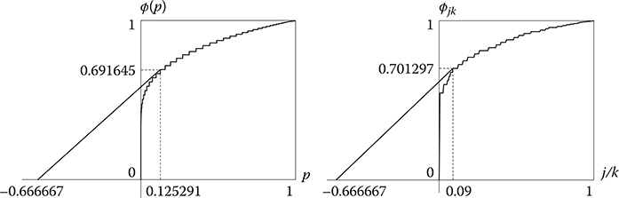
FIGURE 3.5
Determination and estimation of the optimal software rejuvenation schedule under steady-state system availability.

Figure 3.6 shows the asymptotic behavior of estimates of the optimal software rejuvenation schedule and its maximum system availability. In the figure, estimates of $n_{0}^{*}$ and $A ({\hat{n}}_{0}^{*})$ are calculated from the estimation algorithm given in Theorem 6, where the horizontal lines in the figure denote the real optimal solutions. From Figure 3.6, it is seen that the optimal software rejuvenation schedule and its associated system availability can be estimated accurately around k = 20, respectively.

3.7.3 Case of Cost-Effectiveness

The left-hand side of Figure 3.7 illustrates the determination of the optimal software rejuvenation schedule on the two-dimensional graph under the cost-effectiveness criterion. Since $p^{*} = 0.0742365$ has the maximum slope from $(- β_{E}, 0) = (- 0.470588, 0)$ in Figure 3.7, the optimal software rejuvenation schedule is $n_{0}^{*} = {(F_{f} * F_{0})}^{- 1} (0.0742365) = 24$ , and the corresponding cost-effectiveness is $E (24) = 0.246606$ .

Images

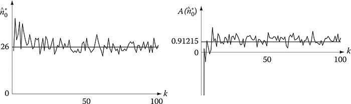
FIGURE 3.6
Asymptotic behavior of estimates of the optimal software rejuvenation schedule and its maximum system availability.

Images

FIGURE 3.7
Determination and estimation of the optimal software rejuvenation schedule under cost-effectiveness.

The right-hand side of Figure 3.7 shows the estimation results of the optimal software rejuvenation schedule. For 200 simulation data, the estimates of the optimal rejuvenation schedule and the maximum cost-effectiveness are given by ${\hat{n}}_{0}^{*} = x_{17} = 25$ and $E ({\hat{n}}_{0}^{*}) = 0.264209$ , respectively.

Figure 3.8 illustrates the asymptotic behavior of estimates of the optimal software rejuvenation schedule and its maximum cost-effectiveness. In the figure, the estimates of $n_{0}^{*}$ and $E ({\hat{n}}_{0}^{*})$ are calculated in accordance with the estimation algorithm given in Theorem 9. From Figure 3.8, it is seen that the optimal software rejuvenation schedule and the cost-effectiveness can be estimated accurately from around k = 20.

3.7.4 Case of Expected Total Discounted Cost

In the expected total discounted cost case, we assume that (r, q = 12, 0.5), $γ = 0.5$ , $c_{s} = 5.0 \times 10 [$ / day]$ , $c_{p} = 3.0 \times 10 [$ / day]$ , $\sum_{y = 0}^{\infty} γ^{y} f_{a} (y) = 0.3$ , $\sum_{s = 0}^{\infty} γ^{s} f_{c} (s) = 0.8,$ and γ = 0.97.

The left-hand side of Figure 3.9 shows the determination of the optimal software rejuvenation schedule on the two-dimensional graph in the case of expected total discounted cost. Since $p^{*} = 0.400808$ has the maximum slope from $(- β_{γ}, - α_{γ}) = (- 0.335878, - 0.202587)$ in Figure 3.9, the optimal software rejuvenation schedule is $n_{0}^{*} = G^{- 1} (0.400808) = 17$ in Eq. (3.49). Then, the corresponding expected total discounted cost over an infinite time horizon is given by TC(17) = 258.939.

The right-hand side of Figure 3.9 presents the estimation results of the optimal software rejuvenation schedule. For 200 simulation data, the estimates of the optimal rejuvenation schedule and its minimum expected total discounted cost are ${\hat{n}}_{0}^{*} = x_{9} = 20$ and $T C ({\hat{n}}_{0}^{*}) = 270.522$ , respectively.

Figure 3.10 illustrates the asymptotic behavior of estimates of the optimal software rejuvenation schedule and its minimum expected total discounted cost. In the figure, the estimates of $n_{0}^{*}$ and $T C ({\hat{n}}_{0}^{*})$ are calculated using Theorem 12. From Figure 3.10, it is seen that the optimal software rejuvenation schedule and the expected total discounted cost can be estimated accurately in rather early phase, respectively.

Images

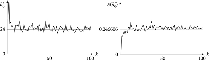
FIGURE 3.8
Asymptotic behavior of estimates of the optimal software rejuvenation schedule and its maximum cost-effectiveness.

Images

FIGURE 3.9
Determination and estimation of the optimal software rejuvenation schedule under expected total discounted cost.

Images

FIGURE 3.10
Asymptotic behavior of estimates of the optimal software rejuvenation schedule and its minimum expected total discounted cost.

3.8 Conclusions

In this chapter, we have summarized optimal periodic software rejuvenation policies in discrete time and their statistical inference approach under the incomplete knowledge of failure time distribution. The key idea is to apply the discrete scaled TTT transform and its numerical counterpart. In this context, the results for expected cost per unit time in the steady state were presented in [46], but the other results for the system availability, cost-effectiveness, and the expected total discounted cost have not been known yet.

In the future, we will consider the discrete models for NPI of software rejuvenation schedule in a similar approach to the references [24, 25 and 26].

References

1. E. Adams, Optimizing preventive service of the software products, IBM Journal of Research & Development, vol. 28, no. 1, pp. 2–14, 1984.

2. A. Avritzer and E.J. Weyuker, Monitoring smoothly degrading systems for increased dependability, Empirical Software Engineering, vol. 2, no. 1, pp. 59–67, 1997.

3. V. Castelli, R.E. Harper, P. Heidelberger, S.W. Hunter, K.S. Trivedi, K.V. Vaidyanathan, and W.P. Zeggert, Proactive management of software aging, IBM Journal of Research & Development, vol. 45, no. 2, pp. 311–332, 2001.

4. M. Grottke, L. Lie, K.V. Vaidyanathan, and K.S. Trivedi, Analysis of software aging in a web server, IEEE Transactions on Reliability, vol. 55, no. 3, pp. 411–420, 2006.

5. A.T. Tai, L. Alkalai, and S.N. Chau, On-board preventive maintenance: a design-oriented analytic study for long-life applications, Performance Evaluation, vol. 35, no. 3, pp. 215–232, 1999.

6. W. Yurcik and D. Doss, Achieving fault-tolerant software with rejuvenation and reconfiguration, IEEE Computer, vol. 18, no. 4, pp. 48–52, 2001.

7. J. Gray and D.P. Siewiorek, High-availability computer systems, IEEE Computer, vol. 24, no. 9, pp. 39–48, 1991.

8. M. Grottke, and K.S. Trivedi, Fighting bugs: Remove, retry, replicate, and rejuvenate, IEEE Computer, vol. 40, pp. 107–109, 2007.

9. Y. Huang, C. Kintala, N. Kolettis, and N.D. Fulton, Software rejuvenation: analysis, module and applications, in Proceedings of the 25th International Symposium on Fault Tolerant Computing (FTC-1995), pp. 381–390, IEEE CPS, 1995.

10. T. Danjou, T. Dohi, N. Kaio, and S. Osaki, Analysis of periodic software rejuvenation policies based on net present value approach, International Journal of Reliability, Quality and Safety Engineering, vol. 11, no. 4, pp. 313–327, 2004.

11. T. Dohi, K. Goseva-Popstojanova, and K.S. Trivedi, Analysis of software cost models with rejuvenation, in Proceedings of the 5th IEEE International Symposium on High Assurance Systems Engineering (HASE-2000), pp. 25–34, IEEE CPS, 2000.

12. T. Dohi, K. Goseva-Popstojanova, and K.S. Trivedi, Statistical non-parametric algorithms to estimate the optimal software rejuvenation schedule, in Proceedings of 2000 Pacific Rim International Symposium on Dependable Computing (PRDC-2000), pp. 77–84, IEEE CPS, 2000.

13. T. Dohi, T. Danjou, and H. Okamura, Optimal software rejuvenation policy with discounting, in Proceedings of 2001 Pacific Rim International Symposium on Dependable Computing (PRDC-2001), pp. 87–94, IEEE CPS, 2001.

14. T. Dohi, K. Goseva-Popstojanova, and K.S. Trivedi, Estimating software rejuvenation schedule in high assurance systems, The Computer Journal, vol. 44, no. 6, pp. 473–485, 2001.

15. T. Dohi, H. Suzuki, and S. Osaki, Transient cost analysis of non-Markovian software systems with rejuvenation, International Journal of Performability Engineering, vol. 2, no. 3, pp. 233–243, 2006.

16. S. Garg, M. Telek, A. Puliafito, and K.S. Trivedi, Analysis of software rejuvenation using Markov regenerative stochastic Petri net, in Proceedings of 6th International Symposium on Software Reliability Engineering (ISSRE-1995), pp. 24–27, IEEE CPS, 1995.

17. H. Suzuki, T. Dohi, K. Goseva-Popstojanova, and K.S. Trivedi, Analysis of multi-step failure models with periodic software rejuvenation, in Advances in Stochastic Modelling (eds., J.R. Artalejo and A. Krishnamoorthy), pp. 85–108, Notable Publications, Neshanic Station, NJ, 2002.

18. T. Dohi, H. Okamura, and K.S. Trivedi, Optimizing software rejuvenation policies under interval reliability criteria, in Proceedings of the 9th IEEE International Conference on Autonomic and Trusted Computing (ATC-2012), pp. 478–485, IEEE CPS, 2012.

19. J. Zhao, W.B. Wang, G.R. Ning, K.S. Trivedi, R. Matias Jr., and K.Y. Cai, A comprehensive approach to optimal software rejuvenation, Performance Evaluation, vol. 70, no. 11, pp. 917–933, 2013.

20. K. Rinsaka and T. Dohi, Optimizing software rejuvenation schedule based on the kernel density estimation, Quality Technology & Quantitative Management, vol. 6, no. 1, pp. 55–65, 2009.

21. R.P.W. Duin, On the choice of smoothing parameters for Parzen estimators of probability density functions, IEEE Transactions on Computers, vol. C-25, no. 11, pp. 1175–1179, 1976.

22. E. Parzen, On the estimation of a probability density function and the mode, Annals of Mathematical Statistics, vol. 33, no. 3, pp. 1065–1076, 1962.

23. B.W. Silverman, Density Estimation for Statistics and Data Analysis, Chapman & Hall, London, 1986.

24. K. Rinsaka and T. Dohi, Non-parametric predictive inference of preventive rejuvenation schedule in operational software systems, in Proceedings of the 18th International Symposium on Software Reliability Engineering (ISSRE-2007), pp. 247–256, IEEE CPS, 2007.

25. K. Rinsaka and T. Dohi, Toward high assurance software systems with adaptive fault management, Software Quality Journal, vol. 24, pp. 65–85, 2016.

26. K. Rinsaka and T. Dohi, An adaptive cost-based software rejuvenation scheme with nonparameteric predictive inference approach, Journal of the Operations Research Society of Japan, vol. 60, no. 4, pp. 461–478, 2017.

27. F.P.A. Coolen and K.J. Yan, Nonparametric predictive inference with right-censored data, Journal of Statistical Planning and Inference, vol. 126, no. 1, pp. 25–54, 2004.

28. P. Coolen-Schrijner and F.P.A. Coolen, Adaptive age replacement strategies based on nonparametric predictive inference, Journal of the Operational Research Society, vol. 55, pp. 1281–1189, 2004.

29. K.V. Vaidyanathan and K.S. Trivedi, A comprehensive model for software rejuvenation, IEEE Transactions on Dependable and Secure Computing, vol. 2, no. 2, pp. 124–137, 2005.

30. Y. Bao, X. Sun, and K.S. Trivedi, Adaptive software rejuvenation: degradation model and rejuvenation scheme, in Proceedings of 33rd Annual IEEE/IFIP International Conference on Dependable Systems and Networks (DSN-2003), pp. 241–248, IEEE CPS, 2003.

31. Y. Bao, X. Sun, and K.S. Trivedi, A workload-based analysis of software aging, and rejuvenation, IEEE Transactions on Reliability, vol. 54, no. 3, pp. 541–548, 2005.

32. A. Bobbio, M. Sereno, and C. Anglano, Fine grained software degradation models for optimal rejuvenation policies, Performance Evaluation, vol. 46, no. 1, pp. 45–62, 2001.

33. H. Okamura, H. Fujio, and T. Dohi, Fine-grained shock models to rejuvenate software systems, IEICE Transactions on Information and Systems (D), vol. E86-D, no. 10>, pp. 2165–2171, 2003.

34. D. Wang, W. Xie, and K.S. Trivedi, Performability analysis of clustered systems with rejuvenation under varying workload, Performance Evaluation, vol. 64, no. 3, pp. 247–265, 2007.

35. W. Xie, Y. Hong, and K.S. Trivedi, Analysis of a two-level software rejuvenation policy, Reliability Engineering and System Safety, vol. 87, no. 1, pp. 13–22, 2005.

36. S. Pfening, S. Garg, A. Puliafito, M. Telek, and K.S. Trivedi, Optimal rejuvenation for tolerating soft failure, Performance Evaluation, vol. 27/28, no. 4, pp. 491–506, 1996.

37. S. Garg, A. Puliafito, M. Telek, and K.S. Trivedi, Analysis of preventive maintenance in transactions based software systems, IEEE Transactions on Computers, vol. 47, pp. 96–107, 1998.

38. H. Okamura, S. Miyahara, T. Dohi, and S. Osaki, Performance evaluation of workload-based software rejuvenation schemes, IEICE Transactions on Information and Systems (D), vol. E84-D, no. 10, pp. 1368–1375, 2001.

39. H. Okamura, S. Miyahara, and T. Dohi, Dependability analysis of a transaction-based multi-server system with rejuvenation, IEICE Transactions on Fundamentals of Electronics, Communications and Computer Sciences (A), vol. E86-A, no. 8, pp. 2081–2090, 2003.

40. H. Okamura, S. Miyahara, and T. Dohi, Rejuvenating communication network system with burst arrival, IEICE Transactions on Communications (B), vol. E88-B, no. 12, pp. 4498–4506, 2005.

41. J. Zheng, H. Okamura, L. Li, and T. Dohi, A comprehensive evaluation of software rejuvenation policies for transaction systems with Markovian arrivals, IEEE Transactions on Reliability, vol. 66, no. 4, pp.1157–1177, 2017.

42. A.P.A. van Moorsel and K. Wolter, Analysis of restart mechanisms in software systems, IEEE Transactions on Software Engineering, vol. 32, no. 8, pp. 547–558, 2006.

43. T. Dohi, K. Iwamoto, H. Okamura, and N. Kaio, Discrete availability models to rejuvenate a telecommunication billing application, IEICE Transactions on Communications (B), vol. E86-B, no. 10, pp. 2931–2939, 2003.

44. K. Iwamoto, T. Dohi, H. Okamura, and N. Kaio, Discrete-time cost analysis for a telecommunication billing application with rejuvenation, Computers & Mathematics with Applications, vol. 51, no. 2, pp. 335–344, 2006.

45. K. Iwamoto, T. Dohi, and N. Kaio, Estimating discrete-time periodic software rejuvenation schedules under cost effectiveness criterion, International Journal of Reliability, Quality and Safety Engineering, vol. 13, no. 6, pp. 565–580, 2006.

46. K. Iwamoto, T. Dohi, and N. Kaio, Estimating periodic software rejuvenation schedule in discrete operational circumstance, IEICE Transactions on Information and Systems (D), vol. E91-D, no. 1, pp. 23–31, 2008.

..................Content has been hidden....................

You can't read the all page of ebook, please click here login for view all page.

Table of Contents for
3. Optimal Periodic Software Rejuvenation Policies in Discrete Time—Survey and Applications

3

Optimal Periodic Software Rejuvenation Policies in Discrete Time—Survey and Applications

CONTENTS

3.1 Introduction

3.2 Model Description

3.2.1 Notation

3.2.2 Model Description

3.3 Expected Cost Analysis

3.3.1 Formulation

3.3.2 Statistical Inference

3.4 Availability Analysis

3.4.1 Formulation

3.4.2 Statistical Inference

3.5 Cost-Effectiveness Analysis

3.5.1 Formulation

3.5.2 Statistical Inference

3.6 Expected Total Discounted Cost Analysis

3.6.1 Formulation

3.6.2 Statistical Inference

3.7 Numerical Examples

3.7.1 Case of Expected Cost

3.7.2 Case of System Availability

3.7.3 Case of Cost-Effectiveness

3.7.4 Case of Expected Total Discounted Cost

3.8 Conclusions

References

Table of Contents for 3. Optimal Periodic Software Rejuvenation Policies in Discrete Time—Survey and Applications

Create new playlist

Sign In

Sign Up

CONTENTS

Table of Contents for
3. Optimal Periodic Software Rejuvenation Policies in Discrete Time—Survey and Applications