
4
Potential Applications of Multivariate Analysis for Modeling the Reliability of Repairable Systems—Examples Tested
Miguel Angel Navas, Carlos Sancho, and Jose Carpio
Spanish National Distance Education University
CONTENTS
4.1 Introduction: Background and Driving Forces
4.2 Study of the Reliability of the System with Methods of IEC Standards
4.3 The Complex Nature of Failures
4.4 Three-Dimensional Graphical Representation of z(t) of the Repairable System
4.5 Potential Multivariate Applications for the Reliability Analysis of Repairable Systems
4.7 Principal Component Analysis
4.1 Introduction: Background and Driving Forces
In the last few decades, the scientific community has developed various statistical methodologies for analysis and modeling of the reliability of repairable systems. The most widely used and accepted methods have been collected by the International Electrotechnical Commission (IEC) in its TC56 technical committee “Dependability,” which has published standards for the European region, taking into account military manuals (MIL-HDBK) issued by the Department of Defense of the United States of America.
The applicable statistical methods and analysis procedures are included in IEC 60300-3-5 (2001). The failure intensity z(t) of a repairable item can be estimated using the successive time between failures (TBF), by means of a stochastic process (SP). If TBF shows no trend and is distributed exponentially, z(t) is constant, and in this case it can be modeled by a homogenous Poisson process (HPP). In cases where there is a trend in z(t), a nonhomogeneous Poisson process (NHPP) can be applied, through a power-law process (PLP).
The IEC 60605-6 developed procedures to determine whether or not a trend in z(t) exists using the U statistic, both for a repairable system and for identical items of repairable systems. If there is no trend in z(t), the point estimation of parameters and confidence intervals is performed with the standard IEC 60605-4. If there is a trend in z(t), the parameters of the PLP model are estimated using the IEC 61710 standard.
Here, the methodology proposed by the IEC is applied to electric traction systems in three series of trains and one series of escalators, from which operating data were available for a period of more than 10 years. Tests of the electric traction systems of the 5000-4th series of trains are presented, and a complementary multivariate analysis is then proposed to characterize the z(t) obtained and analyze the influence of recurrent failures.
4.2 Study of the Reliability of the System with Methods of IEC Standards
As already mentioned, in the statistical methods developed in the IEC standards, the z(t) of the repairable systems can be estimated using an SP. If there is no trend, IEC standards assume that the failures are distributed exponentially and that the number of failures per unit time can be modeled by HPP “perfect repair” (same as new), in which case z(t) is constant. For cases where there is a trend in z(t), NHPP “minimal repair” (same as old) is applied, with modeling using PLP. This method that is most widely used in the industry and has also been adopted by the IEC was developed by Crow (1975).
The IEC standards do not support renewal process (RP) modeling of “perfect repair” when there is no trend in z(t) and the TBF is not distributed exponentially. The nonexistence of a contrasted trend using the statistic U does not guarantee that the TBF will be distributed exponentially. Nor do they envisage modeling with an alternative NHPP for PLP, for which numerous contributions have been published for the improvement of PLP (Attardi and Pulcini, 2005; Bettini et al., 2007).
The procedures to be used in a railway company should preferably be standardized by independent international bodies, in order to be able to demonstrate objectively the safety of their maintenance processes; see EN 50126-1 (1999) for the specification and demonstration of reliability, availability, maintainability, and security (RAMS).
The recommendations of IEC 60300-3-1 (2003) for the selection of analysis techniques and IEC 61703 (2001) for the use of mathematical expressions are also used here. The investigation was carried out in four underground railway repairable systems:
The electric traction system of 36 trains of the 5000-4th series
The electric traction system of 88 trains of the 2000-B series
The electric traction system of 23 trains of the 8000 series
The system of 40 escalators of the TNE model
The traction systems of the trains are composed of repairable items. In the case of failure of an item, for example, a traction motor, the item is removed for repair and once repaired is reassembled on a train. The traction systems are predominantly electric and electronic.
The repairs performed on these systems usually involve the exchange of a damaged component with another, with the assumption that this repair will restore the system to its initial operating state, that is, a “perfect repair.” RP models (including the HPP) are most suitable for a priori use to model reliability (Figure 4.1).
The results of tests on the electric traction systems of the 5000-4th series trains are presented in this chapter (note that the results and conclusions of the same tests carried out on the other three repairable systems were very similar).
The previous studies on the reliability of repairable railway systems using alternative models to SPs include the work of Anderson and Peters (1993) in locomotives; Yongqin and Xishi (1996) in an automatic train protection (ATP) system; Bozzo et al. (2003), Sagareli (2004), and Chen et al. (2007) in AC traction systems. For studies using SP models, see the work of Panja and Ray (2007) on signaling and Luo et al. (2010) on brake control.
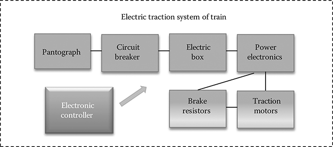
FIGURE 4.1
Repair blocks of an electric traction system.
For electric traction systems, distance in kilometers (km) can be used as a variable instead of time (t) for reliability studies, since the full operation of traction systems depends on the train having traveled some distance, not on the passage of time itself. For example, Anderson and Peters (1993) used kilometers in their study, as traction systems are subjected to wear and tear by the mileage covered.
In the traction systems of 36 trains of the 5000-4th series studied, the records of failures corresponded to the period 1993–2008, that is, 16 years of commercial use. The mileage accumulated for each train exceeded 1,500,000 km. The total number of failures recorded during the study period was 3,112 (Table 4.1).
There is an important and detailed database existing in the railway company, which ensures that the results obtained in the statistical analyses have a high degree of integrity.
In this study, first we attempt to model the reliability of the traction systems of the trains, by means of the estimation of parameters for multiple items, using a single estimation to explain the behavior of the failures of the totality of each system. If this approach fails, the analysis is performed item by item, that is, for each train independently, in order to model the reliability obtained in each train in concrete terms, as recommended by IEC standards. This procedure was also described by Rigdon and Basu (2000).
TABLE 4.1
Summary of Failure Data of Traction Items in 5000-4th Trains

The U-test for multiple items is then applied under IEC 60605-6 (2007) in Section 7.3. With ri the total number of failures to consider from the ith item, Ti* the total time (or km) of the test for the ith item, Tij the time (or km) accumulated at the jth failure of the ith item, and k the total number of items:
The U statistic (Laplace test) is distributed approximately, according to a distribution typified by average 0 and deviation 1. The U statistic can be used to test whether there is evidence of positive or negative growth of reliability, independent of its pattern of growth.
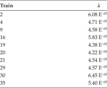
A bilateral test for positive or negative growth with significance level α has critical values u1−α/2 and −u1−α/2, where u1−α/2 is the (1−α/2)100% percentile of the typical normal distribution. If −u1−α/2 < U < u1−α/2, then there is no evidence of positive or negative growth of the reliability to a significance level α. In this case, the hypothesis of an exponential distribution of times between successive failures of the HPP is accepted with significance level α. The critical values u1−α/2 and −u1−α/2 correspond to a unilateral test for positive or negative growth, respectively, with significance level α/2. For the significance levels required, there is a choice of critical values from the appropriate table of percentiles for the typical normal distribution, which in this case is 1.64. From Table 4.2, it can be seen that the traction systems of the 5000-4th trains had a trend of high failure growth, according to the general behavior of the electromechanical systems.
Sections 7.2.2 and 7.3.1.1 of IEC 61710 (2013) on multiple items use the following formula for iterative estimation of :
where N is the total number of failures accumulated in the test, k is the total number of items, ti is the time (or km) to the ith failure (i = 1, 2, …, N), and Tj is the total time (or km) of observation for item j = 1, 2, …, k. Then, can be calculated as follows:
TABLE 4.2
Results of the Trend Test U for the Set of Items in the System
System | U | Ucritical | Trend |
Traction 5000-4th | 16.88 | 1.64 | Very growing |
TABLE 4.3
Results of System Parameter Estimation with the PLP Model
System | β | λ | Trend |
Traction 5000-4th | 1.235 | 1.87 E−06 | Very growing |
TABLE 4.4
Results of Goodness-of-fit Test of the System with the PLP Model
System | C2 | C20,90(M) | PLP Model |
Traction 5000-4th | 2.108 | 0.173 | Rejected |
The model obtained is for the expected accumulated number of failures up to time t:
Iterative calculation of , followed by calculation of , gives the results shown in Table 4.3.
The goodness-of-fit test given in IEC 61710 (2013) is the Cramér–von Mises statistic C2, with M = N and T = T* for testing completed based on time, and M = N − 1 and T = TN for tests completed to failure:
A critical value of C20.90(M) is selected, with a level of significance of 10% of the tabulated value. If C2 exceeds the critical value C20.90(M), C2 > C20.90(M), then the hypothesis that the PLP model fits the test data must be rejected. When applying the PLP model for multiple items, as described in its Sections 7.2.2 and 7.3.1.1 of the IEC 61710 (2013), the model hypothesis is rejected. As shown in Table 4.4, the PLP model was rejected in the test system, owing to the dispersion of failure data of the traction systems of each train.
Then the models are applied to each of the 36 items, in accordance with the provisions of IEC standards. The following formula from Section 7.2 of IEC 60605-6 (2007) is used (Laplace test):
where r is the total number of failures to be considered, T* is the total time (or km) of testing, and Ti is the time (or km) accumulated at the ith failure. The results obtained are summarized in Table 4.5. For each traction system of the 5000-4th trains, the trend was an increasing number of failures, although some items did not present a trend.
TABLE 4.5
Summary of test results of trend U for each item in the system
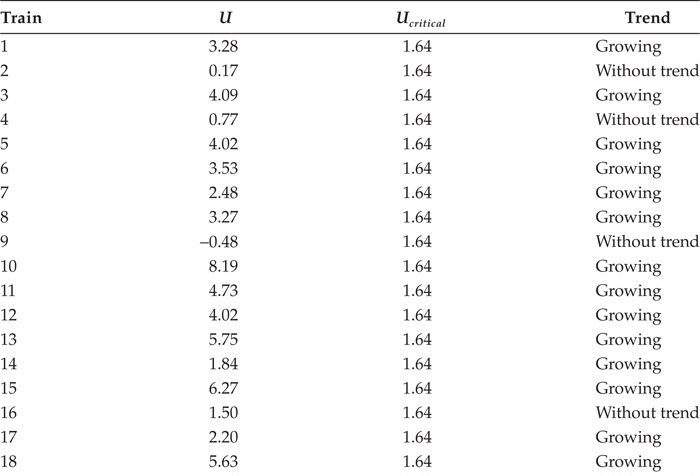
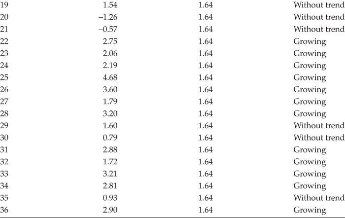
TABLE 4.6
Estimation of λ Constant of Items of Each Traction System of 5000-4th Trains
For each of the ten items without a trend of failure, the λ constant was estimated using the HPP model proposed in the standard IEC 60605-4 (2001), Section 5.1 (see Table 4.6). For tests completed by time (or distance) and repairable items:
where r is the total number of failures to be considered in the test, and T* is the total time (or km) of testing completed at failure. It should be noted that the high degree of dispersion of the constant z (km) obtained between the system items represents unexpected results in traction systems, trains, and operational contexts that are in theory equal.
Finally, the PLP model was applied to each of the 26 items with a trend of failures, according to IEC 61710 (2013), Sections 7.2.1 and 7.3.1.1:
where T* is the total time (or km) of testing and tj is the accumulated time (or km) to the jth failure. Then, unbiased estimates were calculated for and for the completed test as follows:
where N is the total number of accumulated failures in the test, and k is the total number of items in the test. It is necessary to carry out a goodness-of-fit test in order to check whether the model of reliability for each item properly fits the operating data, according to Section 7.3.1.1 of IEC 61710 (2013). The statistic C2 must be calculated with M = N and T = T* for testing based on time (or km):
A critical value of C20.90(M) is selected, with a level of significance of 10% of the tabulated value. If C2 exceeds the critical value C20.90(M), C2> C20.90(M), then the hypothesis that the PLP model fits the test data must be rejected.
The model obtained is for the expected accumulated number of failures up to time t:
and for failure intensity:
A summary of the results is presented in Table 4.7.
The 23 items with a trend of failures could not be modeled using PLP. The PLP model for items with a failure trend generally fails because the TBF does not have an exponential distribution. The following sections will analyze the potential causes of TBF not having an exponential distribution.
For three items with a trend of failures, the model was accepted by a NHPP with the PLP model.
The standard does not collect an NHPP model alternative to PLP for the 23 items with a rejected model. The high rates of models rejected in previous studies have led to the development of multiple models that respond adequately to the results in operation, such as complex SP models and others; see Ruggeri (2006) and Weckman et al. (2001) for examples applied to transport fleets.
4.3 The Complex Nature of Failures
Reliability differences in identical systems operating in equal operating contexts were found in the 36 traction systems of 5000-4th trains, which had reliabilities with different increasing or constant trends.
TABLE 4.7
Estimation of β and λ of the PLP Model of Each Traction System of 5000-4th Trains


Initially, the analysis focused on the search for patterns in the TBF of the systems, observing a generalized trend in which several consecutive failures accumulate during short temporal periods, preceded and followed by long periods without accumulated failures. This phenomenon, termed “recurrent failures,” is well known to those responsible for maintaining repairable systems; see examples in Hatton (1999) and Karanikas (2013).
Subjectively, there is a perception that a series of complex repairable systems (e.g., automobiles) manufactured identically have different reliabilities in practical use. In some cases, studies have corroborated this subjective perception with data showing such disparate values in operation. Indeed, it is usually observed that each item in a set of complex repairable systems does not behave as predicted by a simple reliability model (HPP, NHPP, or RP), and that identical repairable items do not give the same reliability values, with notable differences in some cases.
For this reason, research has been diversified for the development of further models that can adequately represent the reliability of repairable systems. Such investigations were initiated by Lewis (1964), with a branching Poisson process (BPP), and Cox (1972), with a modulated renewal process (MRP). Models of “imperfect repair” include the BP model of Brown and Proschan (1983), the BBS model of Block et al. (1985), the trend renewal process (TRP) of Lindqvist et al. (2003), the generalized renewal processes (GRP) with the concept of “virtual age” introduced by Kijima (1989), and the proportional intensity (PI) models; for comparisons of these models, see Jiang et al. (2005) and Peña (2006). A novel contribution to the GRP model has recently been made by Kaminskiy and Krivtsov (2015). Another approach when the data are correlated is based on frailty models (Peña and Hollander, 2004). At present, more than 100 different models have been developed (Ascher and Feingold, 1984; Pham and Wang 1996; Rigdon and Basu 2000; Guo et al. 2000; Rausand and Hoyland, 2004; Peña, 2006).
Models grouped under the concept of “imperfect,” including those based on SP, try to model the data of repairable systems while taking into account that the repair has not necessarily been “same as new” (perfect repair), nor has it necessarily been “same as old” (minimal repair). Therefore, they include an additional parameter or parameters to modulate the state of restoration to which each repair leads to the repairable item.
In most of these models, the TBF is a random variable with dependent increments, that is, it manifests some degree of relation with another random variable, which may be the previous repair, a preventive maintenance intervention, environmental conditions, etc. If dependence on TBF is demonstrated with some random variable, it statistically invalidates the convenience of using SP models; HPP, HNPP, and RP.
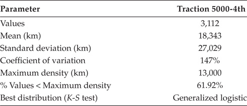
The recurrent failures that a repairable system accumulates during its long operating life are due to different causes, the diagnosis and solution of which may prove difficult in complex systems. Here, TBF data for each system were analyzed, and the most notable results are presented in Table 4.8. A high concentration of TBF can be observed near the origin, which represents recurrent failures. After a certain distance near the repair has been traveled, the distribution of the failures decreases in density. In no case does it correspond to an exponential distribution. The distributions that best represent the TBF sets per system are the generalized logistics for the 5000-4th traction system.
The practical interpretation of these values is that there is a high probability that a failure will occur in the first phases of operation after a repair, after which the probability of failure decreases significantly. Any correlation in the TBF should be ruled out to ensure that the data are independent, and SP models should be applied. This aspect will be analyzed in detail in the following sections, with the application of multivariate analysis.
TABLE 4.8
Basic Parameters of the TBF of Electric Traction Systems of 5000-4th Trains
Also, as the results showed an evident dispersion in the reliability of each item of a system, the analysis of the reliability of the repairable systems may be completed through multivariate technical applications, in order to facilitate decision-making by those in charge of the maintenance of a fleet and/or set of systems consisting of items with disparate reliabilities.
Therefore, recurrent failures are the origin of TBF not having an exponential distribution, depending on the number of repetitive situations of episodes of recurrent failures that each item accumulates during long periods of operation. Recurrent failures substantiate the differences in trend and reliability values between each system item, even if the items are constructively identical and operate in homogeneous contexts.
4.4 Three-Dimensional Graphical Representation of z(t) of the Repairable System
This type of graphics allows the first qualitative identification of the differences between the z(t) of the items under study of each repairable system. Tang and Xie (2002) proposed a dispersion diagram of the λi that are obtained, in order to observe and graphically analyze these differences.
An example of such a graph is shown in Figure 4.2, for the electric traction system of 36 trains of the 5000-4th series, showing ten items with no trend of failure and 26 items with an increasing trend of failures.
Figure 4.2 shows the differences in z (km) obtained for each traction system of 5000-4th-series trains. In the foreground are the z (km) variables corresponding to the traction systems of the 26 trains with increasing model PLP, while in the background are those corresponding to the ten trains with an HPP model, sorted in ascending order (from lowest λi to major λi). This graph also reveals the dispersion of the z (km) of the items and how the values diverge with distance. Up to about 700,000 km, all trains have z (km) within a small range; however, at 1,500,000 km, trains with trends of increasing failures show z (km) values that triplicate to trains with a trend constant of failures.
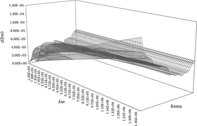
FIGURE 4.2
Three-dimensional graphical representation of the z (km) of traction systems of 5000-4th trains.
4.5 Potential Multivariate Applications for the Reliability Analysis of Repairable Systems
Multivariate analysis is a set of statistical methods whose purpose is to simultaneously analyze multivariate data sets, in the sense that there are several variables measured for each individual or object studied. These statistical methods help the analyst or researcher to make optimal decisions in the context in which they find themselves, taking into account the information available from the data set analyzed. They can be classified into three main groups.
Dependence methods. These suppose that the analyzed variables are divided into two groups: the dependent variables and the independent variables. The purpose of dependence methods is to determine whether and in what way the set of independent variables affects the set of dependent variables.
Methods of interdependence. These methods do not distinguish between dependent and independent variables; their purpose is to identify which variables are related, how they are related, and why.
Structural methods. These assume that the variables are divided into two groups: the dependent variables and the independent variables. The purpose of these methods is to analyze not only how the independent variables affect the dependent variables, but also how the variables of the two groups are related to each other.
Of the existing statistical methods, eight were selected to be tested in the current reliability study of repairable systems, to potentially help and complement the previous modeling tests and results (HPP, NHPP, RP, etc.). Different statistical methods for multivariate analysis have been tested. These include:
Correlations analysis
Principal component analysis
Factor analysis
Cluster analysis
Canonical correlation analysis
Correspondence analysis
Regression analysis
Discriminant analysis
4.6 Correlations Analysis
Correlations analysis measures the strength of the linear relationship between two variables on a scale of −1 to +1. The greater the absolute value of the correlation, the stronger the linear relationship between the two variables. Its application to the reliability of the repairable systems can enable the discovery of dependencies or interdependencies in the TBF, as well as proper selection of the models of reliability that best adapt to the nature of the TBF.
The existence of correlation in the TBF should be ruled out to ensure that the data are independent. The potential variables that could be at the origin of the dependency of TBF in the traction systems were analyzed and evaluated, resulting in 12 variables being studied: train equipment, train alterations, mileage, years of operation, manufacturing date, manufacturing order, driving personnel, maintenance management system, maintenance plan, maintenance personnel, environmental conditions, and railway line. Applied Pearson correlation assays were used to rule out influence on TBF.
Of the 12 variables relating to traction systems of trains, only the results of the 2 variables with appreciable ranges are presented: date of manufacture and manufacturing order. The other ten variables had very similar and/or identical ranges, so that the correlation tests led directly to rejecting the dependency hypothesis with TBF. The influence of seasonality/temperature was ruled out, since the temperature in the tunnels was very stable throughout the year, with a maximum range between 20°C and 30°C. The results of correlations of TBF with context variables in the 5000-4th series trains are presented in Table 4.9.
TABLE 4.9
Correlations of the TBF with Context Variables in 5000-4th Trains


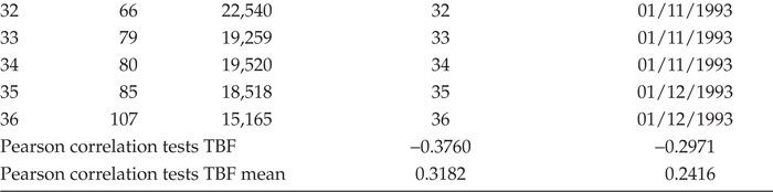
In view of the Pearson correlation values, the influence on the TBF of each traction system of the studied variables could be ruled out. Bredrup et al. (1986) posited decades ago the existence of important differences between the z(t) values obtained in identical systems, and analyzed the influence of nature of the failures: operational, hardware, software, etc.
A correlation study was also carried out on the TBF of each subsystem of the traction systems, and their influence on the TBF of each system, as well as when it was not possible to establish the origin of the failure in any specific part of the system, that is, when no repairs were carried out (only checks). No repairs were carried out were classified as subsystem “without apparent abnormality” (Table 4.10).
As shown in Table 4.11, there was no subsystem with significant correlation with total number of failures, except for “without apparent abnormality” (code 99) failures, and obviously the correlation must be very high, since this group accounts for 48.07% of the total number of failures.
TABLE 4.10
Legend of the Subsystems that Make up the Traction Systems of Trains

TABLE 4.11
Correlations of the Total Failures and Subsystems Failures in 5000-4th Trains
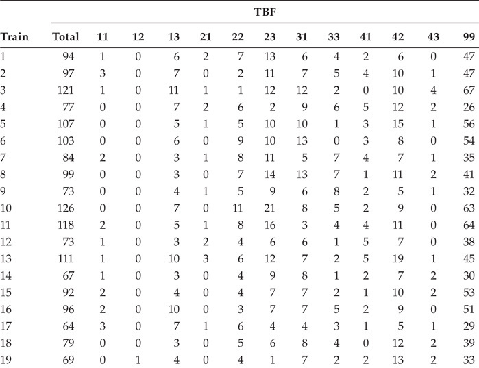

TABLE 4.12
Basic Parameters of the TBF Groups of the 5000-4th Trains

Therefore, it is also necessary to analyze whether the failures with repair “without apparent abnormality” have some degree of correlation with the recurrent failures, since, a priori, there seems to be a cause-effect relationship. That is, when a failure occurs and the repair is completed as “without apparent abnormality,” the failure is likely to be repeated within a few kilometers. The method used for this analysis involves disaggregating and comparing the TBF in two groups: the first group corresponds to the TBF of the failures “without apparent abnormality,” while the second is the remaining TBF in which a repair has been made (Table 4.12).
As shown in Figure 4.3, in the TBF of traction systems of the 5000-4th trains, a high concentration of TBF near the origin can be observed. This represents the recurrent failures, both in the TBF of the “without apparent abnormality” group and in those of the “repaired” group. The TBF densities of both groups are almost identical to each other, as well as to the total TBF of the system. In the traction systems of the 5000-4th series trains, it cannot be said that the recurrent failures have their origin in repairs “without apparent abnormality.”

FIGURE 4.3
Density graph of the TBF groups of traction systems of 5000-4th trains.
In view of the results obtained in the repairable system, it cannot be confirmed that there is a cause-effect relationship between a failure that, after review of the system, the maintenance technician classifies as “without apparent abnormality” and potential repetition of the failure, since the groups of TBF “without apparent abnormality” and “with repair” had almost identical distributions in all the systems.
Next, an attempt was made to set a critical TBF value for the identification of episodes with “accumulation of supposedly abnormal failures” and to typify these TBF as recurrent failures. It has been indicated that the distributions that best represent the TBF sets per system are the generalized logistics for the 5000-4th traction system (Table 4.8).
By adjusting the critical value of TBF for a lower tail area to <15%, the resulting TBF is very close to zero or negative. The interpretation of these results is that any small TBF, TBF → 0, is within the expected ranges of its distribution, so these TBF cannot be considered to be atypical.
Another approach is to try to set a critical number of failures per km interval for the identification of episodes with “accumulation of supposedly abnormal failures” and to typify these as recurrent failures. If, for example, in the traction systems of trains, the failures of each train are grouped in intervals of 15,000 km, it is possible to obtain a metric of “grouping” by interval such as that shown in the histogram of Figure 4.4.

FIGURE 4.4
Histogram of accumulated failures in traction systems of 5000-4th trains.
The 15,000 km intervals have a distribution of the number of accumulated failures. In the case of the traction systems of the 5000-4th series trains, this is more suitably fitted to a three-parameter log-normal distribution. When the upper tail area limit was marked by 15%, the critical value was approximately two failures. In the analysis of the intervals with an accumulation of failures equal to or greater than two, corresponding to 693 out of a total of 4,068, it was not possible to observe any distribution depending on the following:
The train
The range in km
Prior or subsequent intervals with accumulation (or not) of failures
Number of failures accumulated in the interval
The graph in Figure 4.5 shows the failures of the traction systems of 32 5000-4th trains, with no apparent recognizable pattern.
In the correlation tests carried out, there was no statistically recognizable pattern in recurrent failures, there were episodes having an identical distribution with respect to km, and there was no apparent association between types of failures or repairs performed, as a consequence of which it is not possible to distinguish in practice between primary failures and supposed secondary failures. The concentration of failures in certain periods is qualitatively observable; it has not been possible to rule out the hypothesis that a failure fi has a behavior independent of the near failure fi−1 that precedes it, and nor has it been possible to prove otherwise. Therefore, it cannot be ruled out that the HPP, NHPP, and RP models may be adequate to calculate and represent the reliability of the repairable system tested.
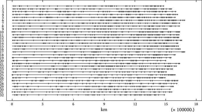
FIGURE 4.5
Graph of failures in 32 items of traction systems of 5000-4th trains.
4.7 Principal Component Analysis
Principal component analysis is designed to extract k major components from a group of p quantitative variables. The main components are defined as a group of linear orthogonal combinations of X having the greatest variance. Determining the major components is often used to reduce the size of a group of predictive variables prior to their use in procedures such as multiple regression or cluster analysis. When variables are highly correlated, the first major components may be sufficient to describe most of the variability present.
In the study of the reliability of repairable systems, this method can be used to find a system or systems that are able to explain the behavior of the set of systems in the evolution of the expected cumulative number of failures E[N(t)].
Principal component analysis of the system tested did not show any train that explains the evolution of the E[N(t)] of the system as a whole. This result was expected, given the dispersion of the E[N(t)] among the items in the system.
4.8 Factor Analysis
The factor analysis procedure is designed to extract m common factors from a group of p quantitative variables X. In many situations, a small number of common factors may be able to represent a large percentage of the variability in the original variables. The ability to express covariates between variables in terms of a small number of significant factors often leads to important questions about the data being analyzed.
Factor analysis may also be used in the study of the reliability of repairable systems to find a system or systems that are able to explain the behavior of the set of systems in the evolution of E[N(t)].
The factor analysis of the system tested did not find any train that could explain the evolution of the E[N(t)] of the system as a whole. Again, this result was expected, given the dispersion of the E[N(t)] among the items in the system.
4.9 Cluster Analysis
The cluster analysis procedure is designed to group observations or variables into groups or clusters based on their similarities. The prime data for the procedure can be in either:
n rows or cases, each containing the values of p quantitative variables
n rows and n columns if observations are grouped, or p rows and p columns if variables are grouped, containing a measure of “distance” between all pairs of items
There are a number of different algorithms for generating groups. Some of the algorithms are agglomerative, starting with separate groups for each observation or variable and then joining them based on their similarity. Other methods begin with a set of “seeds,” and tie other cases or variables to those seeds. In order to create clusters of observations or variables, it is important to have a measure of “closeness” or “similarity” such that similar objects can be joined. When observations are clustered, closeness is typically measured by the distance between observations in the p-dimensional space of variables. The test cluster analysis procedure contains three different metrics for measuring the distance between two objects, represented by x and y:
Square Euclidean distance
Euclidean distance
“City block” distance
When variables are clustered, the distance is similarly defined, except that x and y represent the locations of two variables in the n-dimensional space of observations, and the sum is over observations rather than over variables. The methods tested are as follows:
Agglomerative hierarchical methods: These methods start by putting each observation into a separate cluster. Clusters are linked, two at a time, until the number of clusters is reduced to a desired goal. At each stage, the clusters are paired according to their proximity: nearest neighbor, furthest neighbor, centroid, median, average linkage between groups (UPGMA), and Ward’s method.
k-means method: This method starts by identifying k objects as initial seeds for each cluster. Objects are attached to the nearest cluster.
Cluster analysis may be used in the study of the reliability of repairable systems for the generation of clusters (groups) of repairable systems that have a similar reliability. In many cases, the number of items to be analyzed is very high; the presentation of reliability results for more than 30 systems, for example, can be complex for maintenance management in business organizations. The creation of clusters in repairable systems by selecting outstanding variables of each item simplifies decision-making in such cases. Examples and procedures can be found in the following:
Juarez et al. (2011); variables “dynamic parameters” applied to connection of multi-area power systems
Yu and Chan (2012); variables “temperatures, power and flow” applied to operating performance of chiller systems
Jaafar et al. (2012); variable “driving profiles” applied to the design of railway locomotives
Shang and Wang (2015); variables “reliability, economy, and operational” applied to the power generation group
Rastegari and Mobin (2016); variables “cost, frequency, and downtime” applied to a maintenance management system
In this study, “reliability” is proposed as a variable to simplify maintenance decisions in large fleets. For the creation of clusters in repairable systems without a trend, the values of λi calculated by the HPP reliability models for items without failure trends have been taken as variables. The number of clusters to be generated must be fixed before the test. In the presented results, three clusters have been created:
High cluster: This cluster contains items with high λ that require different maintenance policies, increasing the consistency of preventive maintenance and requiring particular attention to the resolution of failures in corrective maintenance; these are the items with the worst reliability results.
Middle cluster: This cluster contains items with intermediate λ that require regular maintenance policies, with consistent preventive maintenance and the resolution of failures in corrective maintenance.
Low cluster: This cluster contains items with low λ that allow the policies of preventive and corrective maintenance to be relaxed, since these items have the best reliability results.
Cluster analysis was applied using the methods described above. Ward’s method proved to be the most appropriate method for cluster creation, with a balanced number of items and results that were nearly independent of the distance metric used (square Euclidean, Euclidean, and city-block).
As an example, the results of applying this methodology to the 36 traction systems of 5000-4th trains are shown in Figure 4.6. The high cluster consists of seven items, the middle cluster 14, and the low cluster 15. This classification allows maintenance managers to more accurately adjust the different maintenance strategies for groups of items with similar reliability behaviors, in order to use the available resources more efficiently.

FIGURE 4.6
Three clusters of traction systems of 5000-4th trains generated by Ward’s method.
Regardless of the method and metric used to create clusters of items with similar reliabilities in a repairable system, cluster analysis is considered a very useful tool to adjust decisions in maintenance strategies of large fleets, where it would be very complex, although desirable, to perform personalized maintenance for each item according to its reliability at each moment of operation.
4.10 Canonical Correlation Analysis
Canonical correlation analysis is designed to help identify associations between two sets of variables. This is done by finding linear combinations of the variables in the two sets that exhibit strong correlations. The pair of linear combinations with the strongest correlation form the first set of canonical variables. The second set of canonical variables is the pair of linear combinations that show the next strongest correlation, among all combinations that are not correlated with the first set. Frequently, a small number of pairs can be used to quantify the relationship that exists between the two sets.
This method should not be used for the creation of a single “type” individual calculated by the linear combination of the failures of n identical repairable systems, by not having with the necessary statistical support with respect to correct treatment of the TBF, and not contemplate the stochastic nature or dependence of the failures.
4.11 Correspondence Analysis
The correspondence analysis procedure creates a rows-and-columns map in a two-dimensional contingency table to superimpose related categories for row and column variables. However, no more than two or three dimensions are used to show the variability of inertia in the table. An important part of the output is the map of correspondences in which the distance between two categories is a measure of their similarity. No concrete application has been found for this method in the reliability analysis of repairable systems.
4.12 Regression Analysis
The regression analysis procedure is used to construct a statistical model that describes the impact of one or several quantitative factors X1 − Xi, on a dependent variable Y. Multiple models and methods of regression analysis have been developed:
Simple regression
Multiple regression
Logistic regression
Negative binomial regression
Nonlinear regression
Polynomial regression
Poisson regression
Cox proportional hazards
Some of these methods have been used to model the reliability of repairable systems. The most commonly used models have been consolidated in different applied studies; see compendium in Liang (2011):
Exponential smoothing model (ES)
Moving average model (MA)
Autoregressive integrated moving average process, Box-Jenkins ARIMA model
Seasonal autoregressive integrated moving average process, Box-Jenkins SARIMA model
It is important to find the model that best fits the data, without needing to consider the reasons for the behavior of the TBF. An estimation of application of E[N(t)] in different repairable systems by simple regression (least-squares method) is presented. Twenty-seven simple regression models were tested, with or without previous transformation of values of the X-axis (km) and of the Y-axis (E[N(t)]), with the coefficient β0 = 0, since E[N(0)] = 0.
For each item, the regression model that best adapted to the data was selected, that is, the one with a higher of R2 determination coefficient adjusted in a range from 0% to 100%. The goodness-of-fit test was integrated within the ANOVA (analysis of variance) model by decomposing the variability of the dependent variable Y into a sum of squares model of the error or residues. Of particular interest in this analysis is the test F and its associated P-value to test the statistical significance of the adjusted model. A small P-value (less than 0.05 at a significance level of 5%) indicates that a statistical relationship of the specified form exists between Y and X.
Table 4.13 shows the results of applying the simple regression models in E[N(t)] to the traction systems of the 5000-4th trains. Models with limited adjustment to the failures were used. In nine items, the simple regression model that best adjusted was linear (without a trend in the failures), whereas in the tests for trends, the U statistics of these items were positive. Likewise, for each item, the goodness-of-fit test with a significance level of 5% admits between six and nine simple regression models, whose trend is not coincident in some cases, which questions the results and limitations of these simple models.
For the items with no trend in the failures, the most accepted and best fit simple regression model was the linear one, with E[N(t)] = β1 km. As an example, the model for the traction system of train 20 of the 5000-4th series is shown in Figure 4.7. For items with an increasing trend in failures, the most accepted and best fit simple regression model was the square of x, with E[N(t)] = β1 km2. As an example, the model for the traction system of train 1 of the 5000-4th series is shown in Figure 4.8.
Many authors consider this type of model to be unorthodox, since they limit themselves to trying to adjust the data to a mathematical equation, without any explanation or formulation of the nature of the failures and/or their potential origin. This has been verified in the tests presented with these simple mathematical equations.
TABLE 4.13
Estimated Simple Regression Models of E[N(t)] on 5000-4th Trains


FIGURE 4.7
Linear simple regression model of train 20 of the 5000-4th series.

FIGURE 4.8
Square- x simple regression model of train 1 of the 5000-4th series.
4.13 Discriminant Analysis
The discriminant analysis procedure is designed to help distinguish between two or more data groups based on a group of p observed quantitative variables. It does so by constructing discriminant functions that are linear combinations of variables. The purpose of such an analysis is usually one or both of the following:
To be able to describe cases mathematically observed in a way that separates them into groups as best as possible
To be able to classify new observations as belonging to one or other of the groups
No concrete application has been found to this method in the reliability analysis of repairable systems.
4.14 Conclusions
The TBF of items in repairable systems does not necessarily behave in a similar way. Even in what appears to be constructively identical repairable systems, the data may show a great dispersion in their trend and quantitative value of E[N(t)].
The tests carried out showed that in all the repairable systems tested, periods of incremental failures preceded and followed periods without failure. This phenomenon is termed “recurrent failures,” and is the reason why TBF does not have an exponential distribution and there are differences in reliability between constructively identical items and in homogeneous operational contexts.
In the periods of failure increments (recurrent failures), no statistically recognizable pattern was found. These episodes had identical distributions with respect to distance, with no apparent association between types of failures, resulting in primary and secondary failures being indistinguishable.
The items of a repairable system may show dispersed and in many cases divergent reliability values. Multivariate analysis methods may very well be useful to advance knowledge of the nature of the failures and the root causes of the differences in reliability between the items (Table 4.14).
TABLE 4.14
Multivariate Analysis Testing and Application to the Reliability of Repairable Systems

It is proposed that maintenance managers reorient their efforts to study the reliability of each item and not the set, and to implement mechanisms for the proactive detection of episodes of temporary failure increments in each item, applying differential maintenance in each case.
References
Anderson, G.B. and Peters, A.J. (1993), An overview of the maintenance and reliability of AC traction systems, Proceedings of the Joint IEEE/ASME Railroad Conference, pp. 7–15.
Ascher, H. and Feingold, H. (1984), Repairable System Reliability, Marcel Dekker, New York.
Attardi, L. and Pulcini, G. (2005), A new model for repairable systems with bounded failure intensity, IEEE Transactions on Reliability, Vol. 54, No. 4, pp. 572–582.
Bettini, G., Giansante, R. and Tucci, M. (2007), Forecasting fleet warranty returns using modified reliability growth analysis, Proceedings of Annual IEEE Reliability and Maintainability Symposium RAMS’07, pp. 350–355.
Block, H., Borges, W. and Savits, T. (1985), Age-dependent minimal repair, Journal of Applied Probability, Vol. 22, No. 2, pp. 370–385.
Bozzo, R., Fazio, V. and Savio, S. (2003), Power electronics reliability and stochastic performances of innovative AC traction drives: a comparative analysis, 2003 IEEE Bologna Power Tech Conference Proceedings, Vol. 3, pp. 7–14.
Bredrup, E., Evensen, K., Helvik, B.E. and Swensen, A. (1986), The activity-dependent failure intensity of SPC systems—some empirical results, IEEE Journal on Selected Areas in Communications, Vol. 4, No. 7, pp. 1052–1059.
Brown, M. and Proschan, F. (1983), Imperfect repair, Journal of Applied Probability, Vol. 20, No. 4, pp. 851–859.
Chen, S.K., Ho, T.K. and Mao, B.H. (2007), Reliability evaluations of railway power supplies by fault-tree analysis, IET Electric Power Applications, Vol. 1, No. 2, pp. 161–172.
Cox, D.R. (1972), The statistical analysis of dependencies in point process, in Lewis, P.A.W. (Ed.), Symposium on Point Processes, Wiley, New York, pp. 55–66.
Crow, L.H. (1975), Reliability analysis for complex, repairable systems, Technical Report No. 138, AMSAA, Aberdeen, MD.
EN 50126-1 (1999), Railway Applications—The Specification and Demonstration of Reliability. Availability, Maintainability, and Safety (RAMS)-Part, 1. European Committee for Electrotechnical Standardization (CENELEC), Brussels.
Guo, R., Ascher, H. and Love, E. (2000), Generalized models of repairable systems—a survey via stochastic processes formalism, ORiON, Vol. 16, No. 2, pp. 87–128.
Hatton, L. (1999), Repetitive failure, feedback and the lost art of diagnosis, Journal of Systems and Software, Vol. 47, Nos. 2–3, pp. 183–188.
IEC 60300-3-1 ed2.0 (2003), Dependability Management—Part 3-1: Application Guide—Analysis Techniques for Dependability—Guide on Methodology, International Electrotechnical Commission (IEC), Geneva.
IEC 60300-3-5 ed1.0 (2001), Dependability Management—Part 3-5: Application Guide—Reliability Test Conditions and Statistical Test Principles, International Electrotechnical Commission (IEC), Geneva.
IEC 60605-4 ed2.0 (2001), Equipment Reliability Testing—Part 4: Statistical Procedures for Exponential Distribution—Point Estimates, Confidence Intervals, Prediction Intervals and Tolerance Intervals, International Electrotechnical Commission (IEC), Geneva.
IEC 60605-6 ed3.0 (2007), Equipment Reliability Testing—Part 6: Tests for the Validity and Estimation of the Constant Failure Rate and Constant Failure Intensity, International Electrotechnical Commission (IEC), Geneva.
IEC 61703 ed1.0 (2001), Mathematical Expressions for Reliability, Availability, Maintainability and Maintenance Support Terms, International Electrotechnical Commission (IEC), Geneva.
IEC 61710 ed2.0 (2013), Power Law Model—Goodness-of-Fit Tests and Estimation Methods, International Electrotechnical Commission (IEC), Geneva.
Jaafar, A., Sareni, B. and Roboam, X. (2012), Clustering analysis of railway driving missions with niching, COMPEL—The International Journal for Computation and Mathematics in Electrical and Electronic Engineering, Vol. 31, No. 3, pp. 920–931.
Jiang, S.T., Landers, T.L. and Rhoads, T.R. (2005), Semi-parametric proportional intensity models robustness for right-censored recurrent failure data, Reliability Engineering and System Safety, Vol. 90, No. 1, pp. 91–98.
Juarez, C., Messina, A.R., Castellanos, R. and Espinosa-Perez, G. (2011), Characterization of multimachine system behavior using a hierarchical trajectory cluster analysis, IEEE Transactions on Power Systems, Vol. 26, No. 3, pp. 972–981.
Kaminskiy, M. and Krivtsov, V. (2015), Geometric G1-renewal process as repairable system model, Proceedings of Annual IEEE Reliability and Maintainability Symposium, RAMS, Palm Harbor, FL, pp. 1–6.
Karanikas, N. (2013), Using reliability indicators to explore human factors issues in maintenance databases, International Journal of Quality & Reliability Management, Vol. 30, No. 2, pp. 116–128.
Kijima, M. (1989), Some results for repairable systems with general repair, Journal of Applied Probability, Vol. 26, No. 1, pp. 89–102.
Lewis, P. (1964), A branching Poisson process model for the analysis of computer failure patterns, Journal of the Royal Statistical Society Series B (Methodological), Vol. 26, No. 3, pp. 398–456.
Liang, Y. (2011), Analyzing and forecasting the reliability for repairable systems using the time series decomposition method, International Journal of Quality & Reliability Management, Vol. 28, No. 3, pp. 317–327.
Lindqvist, B.H., Elvebakk, G. and Heggland, K. (2003), The trend-renewal process for statistical analysis of repairable systems, Technometrics, Vol. 45, No. 1, pp. 31–44.
Luo, M., Wu, M.L. and Wang, X.Y. (2010), Study on reliability test for brake control execution unit of rail transit vehicle, 2010 International Conference on E-Product, E-Service and E-Entertainment (ICEEE), pp. 1–4.
Panja, S.C. and Ray, P.K. (2007), Reliability analysis of track circuit of Indian railway signalling system, International Journal of Reliability and Safety, Vol. 1, No. 4, pp. 428–445.
Peña, E.A. (2006), Dynamic modeling and statistical analysis of event times, Statistical Science, Vol. 21, No. 4, pp. 487–500.
Peña, E.A. and Hollander, M. (2004), Models for recurrent events in reliability and survival analysis, in Soyer, T., Mazzuchi, T. and Singpurwalla, N. (Eds), Mathematical Reliability: An Expository Perspective, Kluwer Academic Publishers, Dordrecht, pp. 105–123.
Pham, H. and Wang, H. (1996), Imperfect maintenance, European Journal of Operational Research, Vol. 94, No. 3, pp. 425–438.
Rastegari, A. and Mobin, M. (2016), Maintenance decision making, supported by computerized maintenance management system, IEEE 2016 Annual Reliability and Maintainability Symposium (RAMS), pp. 1–8.
Rausand, M. and Hoyland, A. (2004), System Reliability Theory: Models, Statistical Methods, and Applications, 2nd ed., Wiley, New York.
Rigdon, S.E. and Basu, A.P. (2000), Statistical Methods for the Reliability of Repairable Systems, Wiley, New York.
Ruggeri, F. (2006), On the reliability of repairable systems: methods and applications, Proceedings of Progress in Industrial Mathematics at ECMI 2004, pp. 535–553.
Sagareli, S. (2004), Traction power systems reliability concepts, ASME/IEEE 2004 Joint Rail Conference, pp. 35–39.
Shang, L. and Wang, S. (2015), Application of the principal component analysis and cluster analysis in comprehensive evaluation of thermal power units, 5th International Conference on Electric Utility Deregulation and Restructuring and Power Technologies (DRPT), Changsha, pp. 2769–2773.
Tang, L.C. and Xie, M. (2002), A simple graphical approach for comparing reliability trends of different units in a fleet, Proceedings of Annual IEEE Reliability and Maintainability Symposium, Seattle, WA, pp. 40–43.
Weckman, G.R., Shell, R.L. and Marvel, J.H. (2001), Modeling the reliability of repairable systems in the aviation industry, Computers & Industrial Engineering, Vol. 40, Nos. 1–2, pp. 51–63.
Yongqin, H. and Xishi, W. (1996), The reliability and performability of a repairable and degradable ATP system, Vehicular Technology Conference, 1996, Mobile Technology for the Human Race, IEEE 46th, Atlanta, GA, Vol. 3, pp. 1609–1612.
Yu, F.W. and Chan, K.T. (2012), Assessment of operating performance of chiller systems using cluster analysis, International Journal of Thermal Sciences, Vol. 53, pp. 148–155.