12. Reliability and Fault Tolerance Modeling of Multiphase Traction Electric Motors

Nowadays, the complexity of modern engineering systems is increasing. The main function of such systems is to achieve the required level of sustainable and safety operations with maximum efficient and stable fulfillment. The implementation of the specified requirements is closely related to the assessment of sustainable operation indicators of the system.

Ships’ traction systems are the safety-critical systems and their operational sustainability is obligatory. Taking into consideration the ships’ specific operational conditions, the following features of their electric propulsion systems are important: high autonomy of the ships’ operations, availability of structural and functional redundancies, high maintainability of an electric propulsion system, possibility of repair during operation, etc.

As shown in [²], using a multiphase electric motor allows the increase of fault tolerance of safety-critical systems and takes into account the high requirements imposed to its propulsion system. In the present study, the propulsion system of an icebreaking ship, called a multipower source traction drive (MPSTD), with four diesel generators was analyzed [¹]. Such a topological scheme of traction drives is widely used for transporting icebreaking ships and icebreakers.

Except edition and increase the fault tolerance of traction drive, the structural and functional redundancies of components are used. In most cases, given the traction drive’s limitations of weight and dimensions, for example, in aircraft, structural redundancy is not possible; therefore, a functional redundancy option is used.

A promising variant of the practical implementation of the functional redundancy of one of the main components of the traction electric drive is a multiphase electric motor, which is discussed in detail in this chapter. Figure 12.1 schematically shows the stator topology of a fault-tolerant multiphase permanent magnet synchronous motor. The motor phases are not galvanically connected to each other. Each phase is fed from a power source through a multilevel electrical inverter. In this chapter, the electric motors with 3-, 6-, 9-, and 12-phase topologies are considered.

Images

FIGURE 12.1
Stator topology of multiphase traction electric motor.

Many technical systems, such as MPSTDs, are designed to perform their tasks with different performance levels: level of perfect functioning, level with reduced capacity, and complete failure level. Such systems can be described as multistate systems (MSSs). Usually, MSSs are composed of elements that can be multistate themselves. The basic concepts and the recent development of MSS reliability theory can be found in [⁸] and [⁹]. Different approaches have been introduced for the reliability analysis of such systems: direct partial logic derivatives [⁷] and UGF technique [¹¹] for steady-state performance distributions and L_z-transform techniques [⁶] for dynamic MSS reliability analysis. Many technical applications of L_z-transform are presented in [^{3, 4, 5 and 6}] and [¹¹,¹²].

In the present chapter, the L_z-transform approach is applied to a real multistate MPSTD and its availability and performance are analyzed. It was shown that in comparison with the straightforward Markov method, the L_z-transform approach drastically simplifies the computation of the operational sustainability value for such a system.

12.2 Brief Description of the L_z-Transform Method

We consider a MSS, consisting of n multistate components. Any j-component can have k_j different states, corresponding to different performances g_ji, represented by the set $g_{j} = {g_{j 1}, \dots, g_{j k_{j}}}$ , $j = {1, \dots, n}; i = {1, 2, \dots, k_{j}}$ . The performance stochastic processes $G_{j} (t) \in g_{j}$ and the system structure function $G (t) = f (G_{1} (t), \dots, G_{n} (t))$ that produce the stochastic process corresponding to the output performance of the entire MSS fully define the MSS model.

The MSS model definitions can be divided into the following steps. For each multistate component, we will build a model of the stochastic process. The Markov performance stochastic process for each component j can be represented by the expression $G_{j} (t) =$ ${g_{j}, A_{j}, p_{j 0}}$ , where g_j is the set of possible component’s states, defined as follows: $A_{j} = (a_{l m}^{(j)} (t)), l, m = 1, \dots, k; j = 1, \dots, n$ —transition intensities matrix and $p_{j 0} = [p_{10}^{(j)} = \Pr {G_{j} (0) = g_{10}}, \dots, p_{k_{j} 0}^{(j)} = \Pr {G_{j} (0) = g_{k_{j} 0}}]$ —initial states probability distribution.

For each component j, the system of Kolmogorov forward differential equations [⁶] can be written for the determination of the state probabilities $p_{j i} (t) = \Pr {G_{j} (t) = g_{j i}}, i = 1, \dots, k_{j}, j = 1, \dots, n$ under initial conditions $p_{j 0}$ . Now the L_z-transform of a discrete-state continuous-time (DSCT) Markov process G_j(t) for each component j can be written as follows:

$\begin{matrix} L_{Z} {G_{j} (t)} = \sum_{i = 1}^{k_{j}} p_{j i} (t) z^{g_{j i}} . \end{matrix} (12.1)$

In the next step, in order to find L_z-transform of the entire MSS’s output performance Markov Process G(t), the Ushakov’s Universal Generating Operator [¹²] can be applied to all individual L_z-transforms $L_{Z} {G_{j} (t)}$ over all time points t ≥ 0

$\begin{matrix} L_{Z} {G (t)} = Ω_{f} {L_{Z} [G_{1} (t)], \dots, L_{Z} [G_{n} (t)]} = \sum_{i = 1}^{K} p_{i} (t) z^{g_{i}} . \end{matrix} (12.2)$

The technique of Ushakov’s operator application is well established for many different structure functions [⁷].

Using the resulting L_z–transform, MSS’s mean instantaneous availability for the constant demand level w can be derived as the sum of all probabilities in the L_z-transform from terms where powers of z are not negative:

$\begin{matrix} A (t) = \sum_{g_{i} \geq w} p_{i} (t) . \end{matrix} (12.3)$

MSS’s mean instantaneous performance may be calculated as the sum of all probabilities multiplied to performance in the L_z-transform from terms where powers of z are positive:

$\begin{matrix} E (t) = \sum_{g_{i} > 0} p_{i} (t) g_{i} . \end{matrix} (12.4)$

The instantaneous performance deficiency D(t) at any time t for the constant demand w can be calculated as follows:

$\begin{matrix} D (t) = \sum_{g_{i} > 0} p_{i} (t) \cdot max (w - g_{i}, 0) . \end{matrix} (12.5)$

12.3 Multistate Model of the MPSTD

12.3.1 System Description

We analyze a conventional diesel-electric power drive, using it in Amguema-type arctic cargo ships, based on a direct electric propulsion system. The structure of ship’s diesel-electric traction drive is shown in Figure 12.2. The system consists of a diesel-generator subsystem, a main switchboard, an electric energy converter, and an electric motor.

Images

FIGURE 12.2
Structure of the ship’s diesel-electric traction drive.

The energy performance of the whole system is 5500 kW. Depending on the ice conditions, the amount of cargo, and other conditions of navigation, ship’s propulsion system is operating with a different number of diesel and electric propulsion motors. It realizes the required value of the performance and, as a consequence, the high survivability of the ship with the possible occurrence of critical failures of power equipment.

The power-generating performance of each diesel generator is 1375 kW. Therefore, connecting a diesel generator in parallel supports the nominal generating performance, which is required for the functioning of the whole system.

The main switchboard device, the electric energy converter, and the electric motor have the nominal performance.

In the ship’s diesel-electric power drives with a fix pitch propeller, the dimensions of the electric machines have to be calculated accurately in order to estimate the available sufficient propulsion power, which is directly determined by the required value of operational power and needed additional power in case of heavy weather or ice conditions in the area of navigation. Possible structures of the arctic ship’s propulsion system with a different number of diesel generators and main traction motors are determined by operating conditions of the arctic ship and the ice and temperature conditions.

The typical operational modes of arctic cargo ships are as follows:

Navigation with icebreaker in heavy ice and navigation without icebreaker in solid ice need 100% of the generated power.
Navigation in the open water depended on the required velocity needs 75% of the generated power.

Images

FIGURE 12.3
Reliability block diagram of the ship’s diesel-electric traction drive.

As an alternative to the conventional 3-phase traction electric motor, a multiphase traction motor with 6-, 9-, and 12-phases is considered, the detailed description and features of which are presented in [²]. The reliability block diagram of the whole ship’s traction drive is shown in Figure 12.3.

12.3.2 Element Description

For system’s elements, which have two states (fully working and fully failed), in order to calculate the probabilities of each state we build the state-space diagram (Figure 12.4) and the following system of differential equations:

${\begin{cases} \frac{d p_{i 1} (t)}{d t} = - λ_{i} p_{i 1} (t) + μ_{i} p_{i 2} (t), \\ \frac{d p_{i 2} (t)}{d t} = λ_{i} p_{i 1} (t) - μ_{i} p_{i 2} (t) \end{cases}$

where i =DE, G, MS, EEC.

Initial conditions are $p_{i 1} (0) = 1; p_{i 2} (0) = 0 .$

We used MATLAB^® for the numerical solution of these systems of differential equations to obtain the probabilities $p_{i 1} (t), p_{i 2} (t)$ (i =DE, G, MS, EEC). Therefore, for such system’s element the output performance stochastic processes can be obtained as follows:

Images

FIGURE 12.4
State-space diagram of elements with two states.

${\begin{cases} g_{i} = {g_{i 1}, g_{i 1}} = {1375, 0}, \\ p_{i} (t) = {p_{i 1} (t), p_{i 1} (t)} . \end{cases}$

Sets $g_{i}, p_{i} (t)$ (i =DE, G, MS, EEC) define L_z-transforms for each element as follows:

Diesel engine:

$\begin{matrix} L_{z} {g^{D E} (t)} = p_{1}^{D E} (t) z^{g_{1}^{D E}} + p_{2}^{D E} (t) z^{g_{2}^{D E}} = p_{1}^{D E} (t) z^{1375} + p_{2}^{D E} (t) z^{0} . \end{matrix} (12.6)$

Generator:

$\begin{matrix} L_{z} {g^{G} (t)} = p_{1}^{G} (t) z^{g_{1}^{G}} + p_{2}^{G} (t) z^{g_{2}^{G}} = p_{1}^{G} (t) z^{1375} + p_{2}^{G} (t) z^{0} . \end{matrix} (12.7)$

Main switchboard:

$\begin{matrix} L_{z} {g^{M S} (t)} = p_{1}^{M S} (t) z^{g_{1}^{M S}} + p_{2}^{M S} (t) z^{g_{2}^{M S}} = p_{1}^{M S} (t) z^{5500} + p_{2}^{M S} (t) z^{0} . \end{matrix} (12.8)$

Electric energy converter:

$\begin{matrix} L_{z} {g^{E E C} (t)} = p_{1}^{E E C} (t) z^{g_{i 1}^{E E C}} + p_{2}^{E E C} (t) z^{g_{i 2}^{E E C}} = p_{1}^{E E C} (t) z^{5500} + p_{2}^{E E C} (t) z^{0} . \end{matrix} (12.9)$

The system’s element, three-phase motor, has three states: fully working state with performance of 5500 kW, partial failure state with performance of 3667 kW, and full failure. The state-space diagram is presented in Figure 12.5. To calculate the probabilities of each state, we build the following system of differential equations:

Images

FIGURE 12.5
State-space diagram of three-phase motor.

${\begin{cases} \frac{d p_{1}^{M_{3}} (t)}{d t} = - λ_{M} p_{1}^{M_{3}} (t) + μ_{M} (p_{2}^{M_{3}} (t) + p_{3}^{M_{3}} (t)), \\ \frac{d p_{2}^{M_{3}} (t)}{d t} = λ_{M} p_{1}^{M_{3}} (t) - (λ_{M} + μ_{M}) p_{2}^{M_{3}} (t) \\ \frac{d p_{3}^{M_{3}} (t)}{d t} = λ_{M} p_{2}^{M_{3}} (t) - μ_{M} p_{3}^{M_{3}} (t) . \end{cases}$

The initial conditions are as follows:

$p_{1}^{M_{3}} (0) = 1; p_{2}^{M_{3}} (0) = 0; p_{3}^{M_{3}} (0) = 0 .$

We used MATLAB^® for numerical solution of this system of differential equations to obtain the probabilities $p_{1}^{M_{3}} (t), p_{2}^{M_{3}} (t), p_{3}^{M_{3}} (t) .$ Therefore, for such system’s element the output performance stochastic processes can be obtained as follows:

${\begin{cases} g^{M_{3}} = {g_{1}^{M_{3}}, g_{2}^{M_{3}}, g_{3}^{M_{3}}} = {5500, 3670, 0}, \\ p^{M_{3}} (t) = {p_{1}^{M_{3}} (t), p_{2}^{M_{3}} (t), p_{3}^{M_{3}} (t)} . \end{cases}$

Sets $g^{M_{3}}, p^{M_{3}} (t)$ define L_z-transforms for three-phase Motor as follows:

$\begin{matrix} L_{z} {g^{M_{3}} (t)} & = & p_{1}^{M_{3}} (t) z^{g_{1}^{M_{3}}} + p_{2}^{M_{3}} (t) z^{g_{2}^{M_{3}}} + p_{3}^{M_{3}} (t) z^{g_{3}^{M_{3}}} \\ = & p_{1}^{M_{3}} (t) z^{5500} + p_{2}^{M_{3}} (t) z^{3670} + p_{3}^{M_{3}} (t) z^{0} . \end{matrix} (12.10)$

The system’s element, six-phase motor, has four states: fully working state with performance 5500 kW, partial failure states with performances 4583 and 3670 kW, and full failure. The state-space diagram is presented in Figure 12.6. To calculate the probabilities of each state we build the following system of differential equations:

Images

FIGURE 12.6
State-space diagram of six-phase motor.

${\begin{cases} \frac{d p_{1}^{M_{6}} (t)}{d t} = - λ_{M} p_{1}^{M_{6}} (t) + μ_{M} (p_{2}^{M_{6}} (t) + p_{3}^{M_{6}} (t) + p_{4}^{M_{6}} (t)), \\ \frac{d p_{2}^{M_{6}} (t)}{d t} = λ_{M} p_{1}^{M_{6}} (t) - (λ_{M} + μ_{M}) p_{2}^{M_{6}} (t) \\ \frac{d p_{3}^{M_{6}} (t)}{d t} = λ_{M} p_{2}^{M_{6}} (t) - (λ_{M} + μ_{M}) p_{3}^{M_{6}} (t) \\ \frac{d p_{4}^{M_{6}} (t)}{d t} = λ_{M} p_{3}^{M_{6}} (t) - μ_{M} p_{4}^{M_{6}} (t) . \end{cases}$

The initial conditions are as follows:

$p_{1}^{M_{6}} (0) = 1; p_{2}^{M_{6}} (0) = 0; p_{3}^{M_{6}} (0) = 0; p_{4}^{M_{6}} (0) = 0 .$

We used MATLAB^® for numerical solution of this system of differential equations to obtain the probabilities $p_{1}^{M_{6}} (t), p_{2}^{M_{6}} (t), p_{3}^{M_{6}} (t), p_{4}^{M_{6}} (t) .$ Therefore, for such system’s element the output performance stochastic processes can be obtained as follows:

${\begin{cases} g^{M_{6}} = {g_{1}^{M_{6}}, g_{2}^{M_{6}}, g_{3}^{M_{6}}, g_{4}^{M_{6}}} = {5500, 4583, 3670, 0}, \\ p^{M_{6}} (t) = {p_{1}^{M_{6}} (t), p_{2}^{M_{6}} (t), p_{3}^{M_{6}} (t), p_{4}^{M_{6}} (t)} . \end{cases}$

Sets $g^{M_{6}}, p^{M_{6}} (t)$ define L_z-transforms for six-phase Motor as follows:

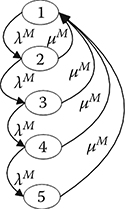
$\begin{matrix} L_{z} {g^{M_{6}} (t)} & = & p_{1}^{M_{6}} (t) z^{g_{1}^{M_{6}}} + p_{2}^{M_{6}} (t) z^{g_{2}^{M_{6}}} + p_{3}^{M_{6}} (t) z^{g_{3}^{M_{6}}} + p_{4}^{M_{6}} (t) z^{g_{4}^{M_{6}}} \\ = & p_{1}^{M_{6}} (t) z^{5500} + p_{2}^{M_{6}} (t) z^{4583} + p_{3}^{M_{6}} (t) z^{3670} + p_{4}^{M_{6}} (t) z^{0} . \end{matrix} (12.11)$

Images

FIGURE 12.7
State-space diagram of nine-phase motor.

The system’s element, nine-phase motor, has five states: fully working state with performance 5500 kW, partial failure states with performances 4889, 4278, and 3670 KW and full failure. The state-space diagram is presented in Figure 12.7. To calculate the probabilities of each state we build the following system of differential equations:

${\begin{cases} \frac{d p_{1}^{M_{9}} (t)}{d t} = - λ_{M} p_{1}^{M_{9}} (t) + μ_{M} (p_{2}^{M_{9}} (t) + p_{3}^{M_{9}} (t) + p_{4}^{M_{9}} (t) + p_{5}^{M_{9}} (t)), \\ \frac{d p_{2}^{M_{9}} (t)}{d t} = λ_{M} p_{1}^{M_{9}} (t) - (λ_{M} + μ_{M}) p_{2}^{M_{9}} (t) \\ \frac{d p_{3}^{M_{9}} (t)}{d t} = λ_{M} p_{2}^{M_{9}} (t) - (λ_{M} + μ_{M}) p_{3}^{M_{9}} (t) \\ \frac{d p_{4}^{M_{9}} (t)}{d t} = λ_{M} p_{3}^{M_{9}} (t) - (λ_{M} + μ_{M}) p_{4}^{M_{9}} (t) \\ \frac{d p_{5}^{M_{9}} (t)}{d t} = λ_{M} p_{4}^{M_{9}} (t) - μ_{M} p_{5}^{M_{9}} (t) . \end{cases}$

The initial conditions are as follows:

$p_{1}^{M_{9}} (0) = 1; p_{2}^{M_{9}} (0) = 0; p_{3}^{M_{9}} (0) = 0; p_{4}^{M_{9}} (0) = 0; p_{5}^{M_{9}} (0) = 0 .$

We used MATLAB^® for numerical solution of this system of differential equations to obtain probabilities $p_{1}^{M_{9}} (t), p_{2}^{M_{9}} (t), p_{3}^{M_{9}} (t), p_{4}^{M_{9}} (t), p_{5}^{M_{9}} (t) .$ Therefore, for such system’s element the output performance stochastic processes can be obtained as follows:

${\begin{cases} g^{M_{9}} = {g_{1}^{M_{9}}, g_{2}^{M_{9}}, g_{3}^{M_{9}}, g_{4}^{M_{9}}, g_{5}^{M_{9}}} = {5500, 4889, 4278, 3670, 0}, \\ p^{M_{9}} (t) = {p_{1}^{M_{9}} (t), p_{2}^{M_{9}} (t), p_{3}^{M_{9}} (t), p_{4}^{M_{9}} (t), p_{5}^{M_{9}} (t)} . \end{cases}$

Sets $g^{M_{9}}, p^{M_{9}} (t)$ define L_z-transforms for a nine-phase motor as follows:

$\begin{matrix} L_{z} {g^{M_{9}} (t)} & = & p_{1}^{M_{9}} (t) z^{g_{1}^{M_{9}}} + p_{2}^{M_{9}} (t) z^{g_{2}^{M_{9}}} + p_{3}^{M_{9}} (t) z^{g_{3}^{M_{9}}} + p_{4}^{M_{9}} (t) z^{g_{4}^{M_{9}}} + p_{5}^{M_{9}} (t) z^{g_{5}^{M_{9}}} \\ = & p_{1}^{M_{9}} (t) z^{5500} + p_{2}^{M_{9}} (t) z^{4889} + p_{3}^{M_{9}} (t) z^{4278} + p_{4}^{M_{9}} (t) z^{3670} + p_{5}^{M_{9}} (t) z^{0} . \end{matrix} (12.12)$

The system’s element, 12-phase motor, has six states: fully working state with performance 5500 kW, partial failure states with performances 5042, 4583, 4125, and 3670 kW, and full failure. The state-space diagram is presented in Figure 12.8. To calculate the probabilities of each state we build the following system of differential equations:

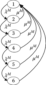
${\begin{cases} \frac{d p_{1}^{M_{12}} (t)}{d t} = - λ_{M} p_{1}^{M_{12}} (t) + μ_{M} (p_{2}^{M_{12}} (t) + p_{3}^{M_{12}} (t) + p_{4}^{M_{12}} (t) + p_{5}^{M_{12}} (t) + p_{6}^{M_{12}} (t)), \\ \frac{d p_{2}^{M_{12}} (t)}{d t} = λ_{M} p_{1}^{M_{12}} (t) - (λ_{M} + μ_{M}) p_{2}^{M_{12}} (t) \\ \frac{d p_{3}^{M_{12}} (t)}{d t} = λ_{M} p_{2}^{M_{12}} (t) - (λ_{M} + μ_{M}) p_{3}^{M_{12}} (t) \\ \frac{d p_{4}^{M_{12}} (t)}{d t} = λ_{M} p_{3}^{M_{12}} (t) - (λ_{M} + μ_{M}) p_{4}^{M_{12}} (t) \\ \frac{d p_{5}^{M_{12}} (t)}{d t} = λ_{M} p_{4}^{M_{12}} (t) - (λ_{M} + μ_{M}) p_{5}^{M_{12}} (t) \\ \frac{d p_{6}^{M_{12}} (t)}{d t} = λ_{M} p_{5}^{M_{12}} (t) - μ_{M} p_{6}^{M_{12}} (t) . \end{cases}$

Images

FIGURE 12.8
State-space diagram of 12-phase motor.

The initial conditions are as follows:

$p_{1}^{M_{12}} (0) = 1; p_{2}^{M_{12}} (0) = p_{3}^{M_{12}} (0) = p_{4}^{M_{12}} (0) = p_{5}^{M_{12}} (0) = p_{6}^{M_{12}} (0) = 0 .$

We used MATLAB^® for numerical solution of this system of differential equations to obtain the probabilities $p_{1}^{M_{12}} (t), p_{2}^{M_{12}} (t), p_{3}^{M_{12}} (t), p_{4}^{M_{12}} (t), p_{5}^{M_{12}} (t),$ $p_{6}^{M_{12}} (t) .$ Therefore, for such system’s element the output performance stochastic processes can be obtained as follows:

${\begin{cases} g^{M_{12}} = {g_{1}^{M_{12}} , g_{2}^{M_{12}}, g_{3}^{M_{12}}, g_{4}^{M_{12}} , g_{5}^{M_{12}}, g_{6}^{M_{12}}} = {5500, 5042, 4583, 4125, 3670, 0}, \\ p^{M_{12}} (t) = {p_{1}^{M_{12}} (t), p_{2}^{M_{12}} (t), p_{3}^{M_{12}} (t), p_{4}^{M_{12}} (t), p_{5}^{M_{12}} (t), p_{6}^{M_{12}} (t)} . \end{cases}$

Sets $g^{M_{12}}, p^{M_{12}} (t)$ define L_z-transforms for nine-phase Motor as follows:

$\begin{matrix} L_{z} {g^{M_{12}} (t)} & = & p_{1}^{M_{12}} (t) z^{g_{1}^{M_{12}}} + p_{2}^{M_{12}} (t) z^{g_{2}^{M_{12}}} + p_{3}^{M_{12}} (t) z^{g_{3}^{M_{12}}} + p_{4}^{M_{12}} (t) z^{g_{4}^{M_{12}}} \\ + p_{5}^{M_{12}} (t) z^{g_{5}^{M_{12}}} + p_{6}^{M_{12}} (t) z^{g_{6}^{M_{12}}} \\ = & p_{1}^{M_{12}} (t) z^{5500} + p_{2}^{M_{12}} (t) z^{5042} + p_{3}^{M_{12}} (t) z^{4583} + p_{4}^{M_{12}} (t) z^{4125} \\ + p_{5}^{M_{12}} (t) z^{3670} + p_{6}^{M_{12}} (t) z^{0} . \end{matrix} (12.13)$

12.3.3 Multistate Model for MPSTD

As is shown in Figure 12.3, the multistate model for MPSTD may be presented as connected in series diesel-generator subsystem, main switchboard, electric energy converter, and electric motor. For simplification, we will calculate the whole-system L_z-transform separately: first, L_z-transform of the Diesel-Generator subsystem, second, L_z-transform of connected in series diesel-generator subsystem, main switchboard, electric energy converter (this subsystem is names subsystem U) and third, whole system with different kinds of electric motors. Therefore, the whole-system L_z-transform is as follows:

$\begin{matrix} L_{z} {G^{MPSTD} (t)} & = & Ω_{f_{s e r}} (L_{z} {G^{D G S} (t)}, L_{z} {G^{M S} (t)}, L_{z} {G^{E E C} (t)}, L_{z} {G^{M} (t)}) \\ = & Ω_{f_{s e r}} (Ω_{f_{s e r}} (L_{z} {G^{D G S} (t)}, L_{z} {G^{M S} (t)}, L_{z} {G^{E E C} (t)}), L_{z} {G^{M} (t)}) \\ = & Ω_{f_{s e r}} (L_{z} {G^{U} (t)}, L_{z} {G^{M} (t)}) . \end{matrix} (12.14)$

12.3.3.1 Diesel-Generator’s Subsystem

A diesel-generator subsystem consists of four identical pairs of diesel engines and generators connected in parallel. Each diesel engine and each generator is a two-state device: power generating performance of a fully operational state is 1375 kW and a total failure corresponds to a capacity of 0.

Using the composition operator $Ω_{f s e r}$ , we obtain the L_z-transform $L_{z} {G^{D G} (t)}$ for each pair of identical diesel engines and generators, connected in series, where the powers of z are found as a minimum of powers of corresponding terms:

$\begin{matrix} L_{z} {G^{D G} (t)} & = & Ω_{f_{s e r}} (g^{D E} (t), g^{G} (t)) \\ = & p_{1}^{D E} (t) p_{1}^{G} (t) z^{1375} + (p_{1}^{D E} (t) p_{2}^{G} (t) + p_{2}^{D E} (t)) z^{0} . \end{matrix} (12.15)$

Using the following notations:

$\begin{array}{l} p_{1}^{D G} (t) = p_{1}^{D E} (t) p_{1}^{G} (t) \\ p_{2}^{D G} (t) = p_{1}^{D E} (t) p_{2}^{G} (t) + p_{2}^{D E} (t), \end{array}$

we obtain the resulting L_z-transform for the diesel-generator subsystem in the following form:

$\begin{matrix} L_{z} {G^{D G} (t)} = p_{1}^{D G} (t) z^{1375} + p_{2}^{D G} (t) z^{0} . \end{matrix} (12.16)$

Using the composition operator $Ω_{f p a r}$ for 4 diesel-generators, connected in parallel, we obtain the L_z_-transform $L_{z} {G^{S y s D G} (t)}$ for the whole diesel-generator subsystem as follows:

$\begin{matrix} L_{z} {G^{D G S} (t)} = Ω_{f_{p a r}} (L_{z} {G^{D G} (t)}, L_{z} {G^{D G} (t)}, L_{z} {G^{D G} (t)}, L_{z} {G^{D G} (t)}) . \end{matrix} (12.17)$

Using notations

$\begin{array}{l} P_{1}^{D G S} (t) = {p_{1}^{D G} (t)}^{4}, \\ P_{2}^{D G S} (t) = 4 \cdot {p_{1}^{D G} (t)}^{3} p_{2}^{D G} (t), \\ P_{3}^{D G S} (t) = 6 \cdot {p_{1}^{D G} (t)}^{2} {p_{2}^{D G} (t)}^{2}, \\ P_{4}^{D G S} (t) = 4 \cdot p_{1}^{D G} (t) {p_{2}^{D G} (t)}^{3}, \\ P_{5}^{D G S} (t) = {p_{2}^{D G} (t)}^{4}, \end{array}$

we obtain the resulting L_z-transform for the whole diesel-generator subsystem in the following form:

$\begin{matrix} L_{z} {G^{D G S} (t)} & = & P_{1}^{D G S} (t) z^{5500} + P_{2}^{D G S} (t) z^{4125} + P_{3}^{D G S} (t) z^{2750} \\ + P_{4}^{D G S} (t) z^{1375} + P_{5}^{D G S} (t) z^{0} . \end{matrix} (12.18)$

12.3.3.2 L_z-transform Subsystem U Calculation

Using the composition operator $Ω_{f s e r}$ for connected in series diesel-generator subsystem, main switchboard, electric energy converter, we obtain the L_z-transform $L_{z} {G^{U} (t)}$ , where the powers of z are found as minimum of powers of corresponding terms:

$\begin{matrix} L_{z} {G^{U} (t)} & = & Ω_{f_{s e r}} (L_{z} {G^{D G S} (t)}, L_{z} {G^{M S} (t)}, L_{z} {G^{E E C} (t)}) \\ = & Ω_{f_{s e r}} (P_{1}^{D G S} (t) z^{5500} + P_{2}^{D G S} (t) z^{4125} + P_{3}^{D G S} (t) z^{2750} + P_{4}^{D G S} (t) z^{1375} \\ + P_{5}^{D G S} (t) z^{0}, p_{1}^{M S} (t) z^{5500} + p_{2}^{M S} (t) z^{0}, p_{1}^{E E C} (t) z^{5500} + p_{2}^{E E C} (t) z^{0}) . \end{matrix} (12.19)$

Using simple algebra calculations of the powers of z as minimum values of powers of corresponding terms, the whole-system L_z-transform expression is as follows:

$\begin{matrix} L_{z} {G^{U} (t)} = P_{1}^{^{U}} (t) z^{5500} + P_{2}^{^{U}} (t) z^{4125} + P_{3}^{^{U}} (t) z^{2750} + P_{4}^{^{U}} (t) z^{1375} + P_{5}^{^{U}} (t) z^{0}, \end{matrix} (12.20)$

where

$\begin{array}{l} P_{1}^{^{U}} (t) = P_{1}^{D G S} (t) p_{1}^{M S} (t) p_{1}^{E E C} (t), \\ P_{2}^{^{U}} (t) = P_{2}^{D G S} (t) p_{1}^{M S} (t) p_{1}^{E E C} (t), \\ P_{3}^{^{U}} (t) = P_{3}^{D G S} (t) p_{1}^{M S} (t) p_{1}^{E E C} (t), \\ P_{4}^{^{U}} (t) = P_{4}^{D G S} (t) p_{1}^{M S} (t) p_{1}^{E E C} (t), \\ P_{5}^{^{U}} (t) = P_{5}^{D G S} (t) p_{1}^{M S} (t) p_{1}^{E E C} (t) + p_{2}^{M S} (t) p_{1}^{E E C} (t) + p_{2}^{E E C} (t) . \end{array}$

12.3.3.3 Multistate Model for MPSTD with Three-Phase Motor

The state-transition diagram of the diesel-electric power drive is presented in Figure 12.9.

Images

FIGURE 12.9
State-transition diagram of the MPSTD with three-phase traction electric motor.

Using the composition operator $Ω_{f s e r}$ for connected in series subsystem U and three-phase motor, we obtain the L_z-transform $L_{z} {G^{S y s M_{3}} (t)}$ , where the powers of z are found as minimum of powers of corresponding terms:

$\begin{matrix} L_{z} {G^{S y s M_{3}} (t)} & = & Ω_{f_{s e r}} (L_{z} {G^{U} (t)}, L_{z} {g^{M_{3}} (t)}) \\ = & Ω_{f_{s e r}} (P_{1}^{^{U}} (t) z^{5500} + P_{2}^{^{U}} (t) z^{4125} + P_{3}^{^{U}} (t) z^{2750} + P_{4}^{^{U}} (t) z^{1375} + P_{5}^{^{U}} (t) z^{0}, \\ p_{1}^{M_{3}} (t) z^{5500} + p_{2}^{M_{3}} (t) z^{3670} + p_{3}^{M_{3}} (t) z^{0}) . \end{matrix} (12.21)$

Using simple algebra calculations of the powers of z, the whole-system L_z-transform expression is as follows:

$\begin{matrix} L_{z} {G^{S y s M_{3}} (t)} & = & \sum_{i = 1}^{6} P_{i}^{^{S y s M_{3}}} (t) z^{g_{i}^{S y s M_{3}}} \\ = & P_{1}^{^{S y s M_{3}}} (t) z^{5500} + P_{2}^{^{S y s M_{3}}} (t) z^{4125} + P_{3}^{^{S y s M_{3}}} (t) z^{3670} \\ + P_{4}^{^{S y s M_{3}}} (t) z^{2750} + P_{5}^{^{S y s M_{3}}} (t) z^{1375} + P_{6}^{^{S y s M_{3}}} (t) z^{0} \end{matrix} (12.22)$

where

$\begin{array}{l} P_{1}^{^{S y s M_{3}}} (t) = P_{1}^{U} (t) p_{1}^{M_{3}} (t), \\ P_{2}^{^{S y s M_{3}}} (t) = P_{2}^{U} (t) p_{1}^{M_{3}} (t), \\ P_{3}^{^{S y s M_{3}}} (t) = (P_{1}^{U} (t) + P_{2}^{U} (t)) p_{2}^{M_{3}} (t), \\ P_{4}^{^{S y s M_{3}}} (t) = P_{3}^{U} (t) (p_{1}^{M_{3}} (t) + p_{2}^{M_{3}} (t)), \\ P_{5}^{^{S y s M_{3}}} (t) = P_{4}^{U} (t) (p_{1}^{M_{3}} (t) + p_{2}^{M_{3}} (t)), \\ P_{6}^{^{S y s M_{3}}} (t) = P_{3}^{M_{3}} (t) + P_{5}^{U} (t) (p_{1}^{M_{3}} (t) + p_{2}^{M_{3}} (t)) . \end{array}$

12.3.3.4 Multistate Model for MPSTD with Six-Phase Motor

The state-transition diagram of the multipower drive is presented in Figure 12.10.

Images

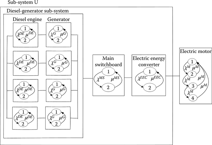
FIGURE 12.10
State-transition diagram of the MPSTD with six-phase traction electric motor.

Using the composition operator $Ω_{f s e r}$ for connected in series subsystem U and six-phase motor, we obtain the L_z-transform $L_{z} {G^{S y s M_{6}} (t)}$ , where the powers of z are found as the minimum of powers of corresponding terms:

$\begin{matrix} L_{z} {G^{S y s M_{6}} (t)} & = & Ω_{f_{s e r}} (L_{z} {G^{U} (t)}, L_{z} {g^{M_{6}} (t)}) \\ = & Ω_{f_{s e r}} (P_{1}^{^{U}} (t) z^{5500} + P_{2}^{^{U}} (t) z^{4125} + P_{3}^{^{U}} (t) z^{2750} + P_{4}^{^{U}} (t) z^{1375} + P_{5}^{^{U}} (t) z^{0}, \\ p_{1}^{M_{6}} (t) z^{5500} + p_{2}^{M_{6}} (t) z^{4583} + p_{3}^{M_{6}} (t) z^{3670} + p_{4}^{M_{6}} (t) z^{0}) . \end{matrix} (12.23)$

The whole-system L_z-transform expression is as follows:

$\begin{matrix} L_{z} {G^{S y s M_{6}} (t)} & = & \sum_{i = 1}^{7} P_{1}^{^{S y s M_{6}}} (t) z^{g_{i}^{S y s M_{6}}} \\ = & P_{1}^{^{S y s M_{6}}} (t) z^{5500} + P_{2}^{^{S y s M_{6}}} (t) z^{4583} + P_{3}^{^{S y s M_{6}}} (t) z^{4125} + P_{4}^{^{S y s M_{6}}} (t) z^{3670} \\ + P_{5}^{^{S y s M_{6}}} (t) z^{2570} + P_{6}^{^{S y s M_{6}}} (t) z^{1375} + P_{7}^{^{S y s M_{6}}} (t) z^{0} \end{matrix} (12.24)$

where

$\begin{array}{l} P_{1}^{^{S y s M_{6}}} (t) = P_{1}^{U} (t) p_{1}^{M_{6}} (t), \\ P_{2}^{^{S y s M_{6}}} (t) = P_{1}^{U} (t) p_{2}^{M_{6}} (t), \\ P_{3}^{^{S y s M_{6}}} (t) = P_{2}^{U} (t) (p_{1}^{M_{6}} (t) + p_{2}^{M_{6}} (t)), \\ P_{4}^{^{S y s M_{6}}} (t) = (P_{1}^{U} (t) + P_{2}^{U} (t)) p_{3}^{M_{6}} (t), \\ P_{5}^{^{S y s M_{6}}} (t) = P_{3}^{U} (t) (1 - p_{4}^{M_{6}} (t)), \\ P_{6}^{^{S y s M_{6}}} (t) = P_{4}^{U} (t) (1 - p_{4}^{M_{6}} (t)), \\ P_{7}^{^{S y s M_{6}}} (t) = p_{4}^{M_{6}} (t) + P_{5}^{U} (t) (1 - p_{4}^{M_{6}} (t)) . \end{array}$

12.3.3.5 Multistate Model for MPSTD with Nine-Phase Motor

The state-transition diagram of the multipower drive is presented in Figure 12.11.

Images

FIGURE 12.11
State-transition diagram of the MPSTD with nine-phase traction electric motor.

Using the composition operator $Ω_{f s e r}$ for connected in series subsystem U and nine-phase motor, we obtain the L_z-transform $L_{z} {G^{S y s M_{9}} (t)}$ , where the powers of z are found as the minimum of powers of corresponding terms:

$\begin{matrix} L_{z} {G^{S y s M_{9}} (t)} & = & Ω_{f_{s e r}} (L_{z} {G^{U} (t)}, L_{z} {g^{M_{9}} (t)}) \\ = & Ω_{f_{s e r}} (P_{1}^{^{U}} (t) z^{5500} + P_{2}^{^{U}} (t) z^{4125} + P_{3}^{^{U}} (t) z^{2750} + P_{4}^{^{U}} (t) z^{1375} + P_{5}^{^{U}} (t) z^{0}, \\ p_{1}^{M_{9}} (t) z^{5500} + p_{2}^{M_{9}} (t) z^{4889} + p_{3}^{M_{9}} (t) z^{4278} + p_{4}^{M_{9}} (t) z^{3670} + p_{5}^{M_{9}} (t) z^{0}) . \end{matrix} (12.25)$

The whole-system L_z-transform expression is as follows:

$\begin{matrix} L_{z} {G^{S y s M_{9}} (t)} & = & \sum_{i = 1}^{8} P_{i}^{^{S y s M_{9}}} (t) z^{g_{i}^{S y s M_{9}}} \\ = & P_{1}^{^{S y s M_{9}}} (t) z^{5500} + P_{2}^{^{S y s M_{9}}} (t) z^{4889} + P_{3}^{^{S y s M_{9}}} (t) z^{4278} + P_{4}^{^{S y s M_{9}}} (t) z^{4125} \\ + P_{5}^{^{S y s M_{9}}} (t) z^{3670} + P_{6}^{^{S y s M_{9}}} (t) z^{2750} + P_{7}^{^{S y s M_{9}}} (t) z^{1375} + P_{8}^{^{S y s M_{9}}} (t) z^{0} \end{matrix} (12.26)$

where

$\begin{array}{l} P_{1}^{^{S y s M_{9}}} (t) = P_{1}^{U} (t) p_{1}^{M_{9}} (t), \\ P_{2}^{^{S y s M_{9}}} (t) = P_{1}^{U} (t) p_{2}^{M_{9}} (t), \\ P_{3}^{^{S y s M_{9}}} (t) = P_{1}^{U} (t) p_{3}^{M_{9}} (t), \\ P_{4}^{^{S y s M_{9}}} (t) = P_{2}^{U} (t) (p_{1}^{M_{9}} (t) + p_{2}^{M_{9}} (t) + p_{3}^{M_{9}} (t)), \\ P_{5}^{^{S y s M_{9}}} (t) = P_{4}^{U} (t) (p_{1}^{M_{9}} (t) + p_{2}^{M_{9}} (t)), \\ P_{6}^{^{S y s M_{9}}} (t) = P_{3}^{U} (t) (1 - p_{5}^{M_{9}} (t)), \\ P_{7}^{^{S y s M_{9}}} (t) = P_{4}^{U} (t) (1 - p_{5}^{M_{9}} (t)), \\ P_{8}^{^{S y s M_{9}}} (t) = p_{5}^{M_{9}} (t) + P_{5}^{U} (t) (1 - p_{5}^{M_{9}} (t)) . \end{array}$

12.3.3.6 Multistate Model for MPSTD with 12-Phase Motor

The state-transition diagram of the multipower drive is presented in Figure 12.12.

Images

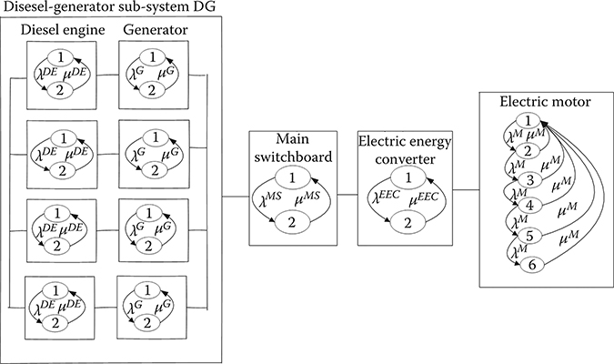
FIGURE 12.12
State-transition diagram of the MPSTD with 12 phase traction electric motor.

Using the composition operator $Ω_{f s e r}$ for connected in series subsystem U and 12-phase motor, we obtain the L_z-transform $L_{z} {G^{S y s M_{12}} (t)}$ , where the powers of z are found as the minimum of powers of corresponding terms:

$\begin{matrix} L_{z} {G^{S y s M_{12}} (t)} & = & Ω_{f_{s e r}} (L_{z} {G^{U} (t)}, L_{z} {g^{M_{12}} (t)}) \\ = & Ω_{f_{s e r}} (P_{1}^{^{U}} (t) z^{5500} + P_{2}^{^{U}} (t) z^{4125} + P_{3}^{^{U}} (t) z^{2750} + P_{4}^{^{U}} (t) z^{1375} + P_{5}^{^{U}} (t) z^{0}, \\ p_{1}^{M_{12}} (t) z^{5500} + p_{2}^{M_{12}} (t) z^{5042} + p_{3}^{M_{12}} (t) z^{4583} + p_{4}^{M_{12}} (t) z^{4125} \\ + p_{5}^{M_{12}} (t) z^{3670} + p_{6}^{M_{12}} (t) z^{0}) . \end{matrix} (12.27)$

The whole-system L_z-transform expression is as follows:

$\begin{matrix} L_{z} {G^{S y s M_{12}} (t)} & = & \sum_{i = 1}^{8} P_{i}^{^{S y s M_{12}}} (t) z^{g_{i}^{S y s M_{12}}} \\ = & P_{1}^{^{S y s M_{12}}} (t) z^{5500} + P_{2}^{^{S y s M_{12}}} (t) z^{5042} + P_{3}^{^{S y s M_{12}}} (t) z^{4583} + P_{4}^{^{S y s M_{12}}} (t) z^{4125} \\ + P_{5}^{^{S y s M_{12}}} (t) z^{3670} + P_{6}^{^{S y s M_{12}}} (t) z^{2750} + P_{7}^{^{S y s M_{12}}} (t) z^{1375} + P_{8}^{^{S y s M_{12}}} (t) z^{0} \end{matrix} (12.28)$

where

$\begin{array}{l} P_{1}^{^{S y s M_{12}}} (t) = P_{1}^{U} (t) p_{1}^{M_{12}} (t), \\ P_{2}^{^{S y s M_{12}}} (t) = P_{1}^{U} (t) p_{2}^{M_{12}} (t), \\ P_{3}^{^{S y s M_{12}}} (t) = P_{1}^{U} (t) p_{3}^{M_{12}} (t), \\ P_{4}^{^{S y s M_{12}}} (t) = P_{2}^{U} (t) (p_{1}^{M_{12}} (t) + p_{2}^{M_{12}} (t) + p_{3}^{M_{12}} (t) + p_{4}^{M_{12}} (t)) + P_{1}^{U} (t) p_{4}^{M_{12}} (t), \\ P_{5}^{^{S y s M_{12}}} (t) = (P_{1}^{U} (t) + P_{2}^{U} (t)) p_{5}^{M_{12}} (t), \\ P_{6}^{^{S y s M_{12}}} (t) = P_{3}^{U} (t) (1 - p_{6}^{M_{12}} (t)), \\ P_{7}^{^{S y s M_{12}}} (t) = P_{4}^{U} (t) (1 - p_{6}^{M_{12}} (t)), \\ P_{8}^{^{S y s M_{12}}} (t) = p_{5}^{U} (t) + P_{6}^{M_{12}} (t) (1 - p_{5}^{U} (t)) . \end{array}$

12.3.4 Calculation Reliability Indices of MPSTD

Using expression (12.3), the MSS instantaneous availability of the MPSTD for different constant demand levels w may be presented as follows:

For 100% demand level (ω = 5500 kW)

$\begin{matrix} \begin{array}{l} A_{w \geq 5500 k W}^{S y s M_{3}} (t) = \sum_{g_{i}^{S y s M_{3}} \geq 5500} P_{i}^{^{S y s M_{3}}} (t) = P_{1}^{^{S y s M_{3}}} (t), \\ A_{w \geq 5500 k W}^{S y s M_{6}} (t) = \sum_{g_{i}^{S y s M_{6}} \geq 5500} P_{i}^{^{S y s M_{6}}} (t) = P_{1}^{^{S y s M_{6}}} (t), \\ A_{w \geq 5500 k W}^{S y s M_{9}} (t) = \sum_{g_{i}^{S y s M_{9}} \geq 5500} P_{i}^{^{S y s M_{9}}} (t) = P_{1}^{^{S y s M_{9}}} (t), \\ A_{w \geq 5500 k W}^{S y s M_{12}} (t) = \sum_{g_{i}^{S y s M_{12}} \geq 5500} P_{i}^{^{S y s M_{12}}} (t) = P_{1}^{^{S y s M_{12}}} (t) . \end{array} \end{matrix} (12.29)$
For 75% demand level (ω = 4125 kW)

$\begin{matrix} \begin{array}{l} A_{w \geq 4125 k W}^{S y s M_{3}} (t) = \sum_{g_{i}^{S y s M_{3}} \geq 4125} P_{i}^{^{S y s M_{3}}} (t) = \sum_{i = 1}^{2} P_{i}^{^{S y s M_{3}}} (t), \\ A_{w \geq 4125 k W}^{S y s M_{6}} (t) = \sum_{g_{i}^{S y s M_{6}} \geq 4125} P_{i}^{^{S y s M_{6}}} (t) = \sum_{i = 1}^{3} P_{i}^{^{S y s M_{6}}} (t), \\ A_{w \geq 4125 k W}^{S y s M_{9}} (t) = \sum_{g_{i}^{S y s M_{9}} \geq 4125} P_{i}^{^{S y s M_{9}}} (t) = \sum_{i = 1}^{4} P_{i}^{^{S y s M_{9}}} (t), \\ A_{w \geq 4125 k W}^{S y s M_{12}} (t) = \sum_{g_{i}^{S y s M_{12}} \geq 4125} P_{i}^{^{S y s M_{12}}} (t) = \sum_{i = 1}^{4} P_{i}^{^{S y s M_{12}}} (t) . \end{array} \end{matrix} (12.30)$

Using expression (12.4), the MSS instantaneous power performance of the MPSTD can be obtained as follows:

$\begin{matrix} E^{S y s M_{3}} (t) & = & \sum_{g_{i}^{S y s M_{3}} > 0} g_{i}^{^{S y s M_{3}}} P_{i}^{^{S y s M_{3}}} (t) = \sum_{i = 1}^{4} g_{i}^{^{S y s M_{3}}} P_{i}^{^{S y s M_{3}}} (t), \\ E^{S y s M_{6}} (t) & = & \sum_{g_{i}^{S y s M_{6}} > 0} g_{i}^{^{S y s M_{6}}} P_{i}^{^{S y s M_{6}}} (t) = \sum_{i = 1}^{6} g_{i}^{^{S y s M_{6}}} P_{i}^{^{S y s M_{6}}} (t), \\ E^{S y s M_{9}} (t) & = & \sum_{g_{i}^{S y s M_{9}} > 0} g_{i}^{^{S y s M_{9}}} P_{i}^{^{S y s M_{9}}} (t) = \sum_{i = 1}^{7} g_{i}^{^{S y s M_{9}}} P_{i}^{^{S y s M_{9}}} (t), \\ E^{S y s M_{12}} (t) & = & \sum_{g_{i}^{S y s M_{9}} > 0} g_{i}^{^{S y s M_{12}}} P_{i}^{^{S y s M_{12}}} (t) = \sum_{i = 1}^{7} g_{i}^{^{S y s M_{12}}} P_{i}^{^{S y s M_{12}}} (t) . \end{matrix} (12.31)$

Using expression (12.5), the instantaneous power deficiency of the MPSTD for different constant demand levels can be presented as follows:

$\begin{matrix} D_{w \geq 5500 k W}^{S y s M_{3}} (t) & = & \sum_{i = 1}^{6} P_{i}^{^{S y s M_{3}}} (t) \cdot max (5500 - g_{i}, 0) \\ = & 1375 \cdot P_{2}^{^{S y s M_{3}}} (t) + 1830 \cdot P_{3}^{^{S y s M_{3}}} (t) + 2750 \cdot P_{4}^{^{S y s M_{3}}} (t) \\ + 4125 \cdot P_{5}^{^{S y s M_{3}}} (t) + 5500 \cdot P_{6}^{^{S y s M_{3}}} (t), \\ D_{w \geq 5500 k W}^{S y s M_{6}} (t) & = & \sum_{i = 1}^{7} P_{i}^{^{S y s M_{6}}} (t) \cdot max (5500 - g_{i}, 0) \\ = & 917 \cdot P_{2}^{^{S y s M_{6}}} (t) + 1375 \cdot P_{3}^{^{S y s M_{6}}} (t) + 1830 \cdot P_{4}^{^{S y s M_{6}}} (t) \\ + 2750 \cdot P_{5}^{^{S y s M_{6}}} (t) + 4125 \cdot P_{6}^{^{S y s M_{6}}} (t) + 5500 \cdot P_{7}^{^{S y s M_{6}}} (t), \\ D_{w \geq 5500 k W}^{S y s M_{9}} (t) & = & \sum_{i = 1}^{8} P_{i}^{^{S y s M_{9}}} (t) \cdot max (5500 - g_{i}, 0) \\ = & 611 \cdot P_{2}^{^{S y s M_{9}}} (t) + 1222 \cdot P_{3}^{^{S y s M_{9}}} (t) + 1375 \cdot P_{4}^{^{S y s M_{9}}} (t) \\ + 1830 \cdot P_{5}^{^{S y s M_{9}}} (t) + 2750 \cdot P_{6}^{^{S y s M_{9}}} (t) + 4125 \cdot P_{7}^{^{S y s M_{9}}} (t) + 5500 \cdot P_{8}^{^{S y s M_{9}}} (t), \\ D_{w \geq 5500 k W}^{S y s M_{12}} (t) & = & \sum_{i = 1}^{8} P_{i}^{^{S y s M_{12}}} (t) \cdot max (5500 - g_{i}, 0) \\ = & 458 \cdot P_{2}^{^{S y s M_{12}}} (t) + 917 \cdot P_{3}^{^{S y s M_{12}}} (t) + 1375 \cdot P_{4}^{^{S y s M_{12}}} (t) \\ + 1830 \cdot P_{5}^{^{S y s M_{12}}} (t) + 2750 \cdot P_{6}^{^{S y s M_{12}}} (t) + 4125 \cdot P_{7}^{^{S y s M_{12}}} (t) \\ + 5500 \cdot P_{8}^{^{S y s M_{12}}} (t), \end{matrix} (12.32)$

$\begin{matrix} D_{w \geq 4125 k W}^{S y s M_{3}} (t) & = & \sum_{i = 1}^{6} P_{i}^{^{S y s M_{3}}} (t) \cdot max (4125 - g_{i}, 0) \\ = & 455 \cdot P_{3}^{^{S y s M_{3}}} (t) + 1375 \cdot P_{4}^{^{S y s M_{3}}} (t) + 2750 \cdot P_{5}^{^{S y s M_{3}}} (t) + 4125 \cdot P_{6}^{^{S y s M_{3}}} (t), \\ D_{w \geq 4125 k W}^{S y s M_{6}} (t) & = & \sum_{i = 1}^{7} P_{i}^{^{S y s M_{6}}} (t) \cdot max (4125 - g_{i}, 0) \\ = & 455 \cdot P_{4}^{^{S y s M_{6}}} (t) + 1375 \cdot P_{5}^{^{S y s M_{6}}} (t) + 2750 \cdot P_{6}^{^{S y s M_{6}}} (t) + 4125 \cdot P_{7}^{^{S y s M_{6}}} (t), \\ D_{w \geq 4125 k W}^{S y s M_{9}} (t) & = & \sum_{i = 1}^{8} P_{i}^{^{S y s M_{9}}} (t) \cdot max (5500 - g_{i}, 0) \\ = & 455 \cdot P_{5}^{^{S y s M_{9}}} (t) + 1375 \cdot P_{6}^{^{S y s M_{9}}} (t) + 2750 \cdot P_{7}^{^{S y s M_{9}}} (t) + 4125 \cdot P_{8}^{^{S y s M_{9}}} (t), \\ D_{w \geq 4125 k W}^{S y s M_{12}} (t) & = & \sum_{i = 1}^{8} P_{i}^{^{S y s M_{12}}} (t) \cdot max (5500 - g_{i}, 0) \\ = & 455 \cdot P_{5}^{^{S y s M_{12}}} (t) + 1375 \cdot P_{6}^{^{S y s M_{12}}} (t) + 2750 \cdot P_{7}^{^{S y s M_{12}}} (t) + 4125 \cdot P_{8}^{^{S y s M_{12}}} (t), \end{matrix} (12.33)$

The failure and repair rates (in year⁻¹) of each system’s elements are presented in Table 12.1 below.

MSS instantaneous availability of the MPSTD for different constant demand levels is presented in Figures 12.13, 12.14, 12.15 and 12.16.

As one can see from Figure 12.13 that the instantaneous availability for 100% demand level is the same for each kind of traction electric motors and after 36.5 days of usage it is 65.2%.

Figure 12.14 shows that the instantaneous availability for 75% demand level is different for each kind of traction electric motors. After 36.5 days of usage, the instantaneous availability for 3-phase traction electric motor is 0.9216, for 6-phase traction electric motors the instantaneous availability is 0.9491, and for 9- and 12-phase traction electric motors the instantaneous availability is 0.95.

TABLE 12.1
Failure and Repair Rates of Each System’s Elements

	Failure Rates (year⁻¹)	Repair Rates (year⁻¹)
Diesel engine	4.99	48.6
Generator	0.2	175
Main switchboard	0.2	440
Electric energy converter	1.5	440
Electric motor	2.7	87.7

Images

FIGURE 12.13
MSS mean instantaneous availability for 100% demand level.

Images

FIGURE 12.14
MSS mean instantaneous availability for 75% demand level.

Comparison instantaneous availability for different demand levels for each kind of traction electric motors is presented in Figures 12.15, 12.16 and 12.17.

Calculated MSS instantaneous power performance of the MPSTD is presented in Figure 12.18.

Calculated MSS instantaneous mean power performance deficiency of the MPSTD is presented in Figures 12.19 and 12.20 and in Table 12.2.

Images

FIGURE 12.15
MSS mean instantaneous availability three-phase motor for different constant demand levels.

Images

FIGURE 12.16
MSS mean instantaneous availability six-phase motors for different constant demand levels.

12.4 Conclusion

In this chapter, the L_z-transform method was used for evaluation of three important parameters of the vehicle’s operational sustainability—availability, performance, and performance deficiency for different kinds of motors of the multistate MPSTD.

Images

FIGURE 12.17
MSS mean instantaneous availability 9- and 12-phase motors for different constant demand levels.

Images

FIGURE 12.18
MSS instantaneous power performance of the MPSTD.

The L_z-transform approach extremely simplifies the solution, which in comparison with the straightforward Markov method would have required building and solving the model with 1072 states for the system with 3-phase motor, 4288 states for the system with 6-phase motor, 5375 states for the system with 9-phase motor, 6400 states for the system with 12-phase motor.

The proposed approach allows optimizing the number of the power sources of traction drive, their characteristics, and schemes of connection in terms of providing the maximum operational sustainability. The results of the calculation allow concluding about the impact of the phase number of the traction electric motor on the reliability and fault tolerance indices of the entire propulsion system. Since the electrical part of the propulsion system is much more reliable than the mechanical part, an increase in the number of phases of traction electric motors does not have a significant effect on the overall performance of the propulsion system. Therefore, to improve the reliability of the entire electric drive, it is advisable to use more reliable combustion engines or their structural redundancy.

Images

FIGURE 12.19
MSS instantaneous mean power performance deficiency for 100% demand level for different kinds of motors of the MPSTD.

Images

FIGURE 12.20
MSS instantaneous mean power performance deficiency for 100% demand level for different kinds of motors of the MPSTD.

TABLE 12.2
MSS Instantaneous Mean Power Performance Deficiency (in kW)

	100% Demand (kW)	75% Demand (kW)
3-Phase motor	578.3	99.8
6-Phase motor	553.8	84.1
9-Phase motor	547.6	83.7
12-Phase motor	544.1	83.7

References

1. I. Bolvashenkov, H.-G. Herzog, Use of stochastic models for operational efficiency analysis of multi power source traction drives, in: Proceedings of the Second International Symposium on Stochastic Models in Reliability Engineering, Life Science and Operations Management, (SMRLO16), I. Frenkel, A. Lisnianski (Eds), 15–18 February 2016, Beer Sheva, Israel, pp. 124–130.

2. I. Bolvashenkov, J. Kammermann, S. Willerich, H.-G. Herzog, Comparative study of reliability and fault tolerance of multi-phase permanent magnet synchronous motors for safety-critical drive trains, in: Proceedings of the International Conference on Renewable Energies and Power Quality (ICREPQ16), 4–6 May 2016, Madrid, Spain, pp. 1–6.

3. I. Frenkel, I. Bolvashenkov, H.-G. Herzog, L. Khvatskin, Performance availability assessment of combined multi power source traction drive considering real operational conditions, Transport and Telecommunication, 2016, 17(3), 179–191.

4. I. Frenkel, I. Bolvashenkov, H.G. Herzog, L. Khvatskin, Operational sustainability assessment of multi power source traction drive, in: Mathematics Applied to Engineering, M. Ram, J.P. Davim (Eds), Elsevier, London, 2017, pp. 191–203.

5. I. Frenkel, I. Bolvashenkov, H.G. Herzog, L. Khvatskin, Lz-transform approach for fault tolerance assessment of various traction drives topologies of hybrid-electric helicopter, in: Recent Advances in Multistate System Reliability: Theory and Applications, In A. Lisnianski, I. Frenkel. A. Karagrigoriou (Eds.), Springer, London, 2017, pp. 321–362.

6. H. Jia, W. Jin, Y. Ding, Y. Song, D. Yu 2017, Multi-state time-varying reliability evaluation of smart grid with flexible demand resources utilizing Lz transform, in: Proceedings of the International Conference on Energy Engineering and Environmental Protection (EEEP2016), IOP Conference Series: Earth and Environmental Science, Vol. 52, 012011, IOP Publishing, Bristol, UK.

7. M. Kvassay, E. Zaitseva, Topological Analysis of Multi-State Systems based on Direct Partial Logic Derivatives, in: Recent Advances in Multistate System Reliability: Theory and Applications, A. Lisnianski, I. Frenkel, & A. Karagrigoriou (Eds), Springer, London, 2018, pp. 265–281.

8. A. Lisnianski, I. Frenkel, Y. Ding, Multi-state System Reliability Analysis and Optimization for Engineers and Industrial Managers, Springer, London, 2010.

9. B. Natvig, Multistate Systems Reliability, Theory with Applications, Wiley, New York, 2011.

10. K. Trivedi, Probability and Statistics with Reliability, Queuing and Computer Science Applications, Wiley, New York, 2002.

11. I. Ushakov, A universal generating function, Soviet Journal of Computer and System Sciences, 1986, 24, 37–49.

12. H. Yu, J. Yang, H. Mo, Reliability analysis of repairable multi-state system with common bus performance sharing, Reliability Engineering and System Safety, 2014, 132, 90–96.

..................Content has been hidden....................

You can't read the all page of ebook, please click here login for view all page.

Table of Contents for
12. Reliability and Fault Tolerance Modeling of Multiphase Traction Electric Motors

12

Reliability and Fault Tolerance Modeling of Multiphase Traction Electric Motors

CONTENTS

12.1 Introduction

12.2 Brief Description of the L_z-Transform Method

12.3 Multistate Model of the MPSTD

12.3.1 System Description

12.3.2 Element Description

12.3.3 Multistate Model for MPSTD

12.3.3.1 Diesel-Generator’s Subsystem

12.3.3.2 L_z-transform Subsystem U Calculation

12.3.3.3 Multistate Model for MPSTD with Three-Phase Motor

12.3.3.4 Multistate Model for MPSTD with Six-Phase Motor

12.3.3.5 Multistate Model for MPSTD with Nine-Phase Motor

12.3.3.6 Multistate Model for MPSTD with 12-Phase Motor

12.3.4 Calculation Reliability Indices of MPSTD

12.4 Conclusion

References

Table of Contents for 12. Reliability and Fault Tolerance Modeling of Multiphase Traction Electric Motors

Create new playlist

Sign In

Sign Up

CONTENTS

Table of Contents for
12. Reliability and Fault Tolerance Modeling of Multiphase Traction Electric Motors