3.1 Introduction

We have used data mining and analytics techniques in several of our efforts for various applications such as social media systems and intrusion detection systems. For example, in our previous book [THUR16], we discussed algorithms for location-based data mining that will extract the locations of the various social media (e.g., Twitter) users. These algorithms can be extended to extract other demographics data. Our prior research has also developed data mining tools for sentiment analysis as well as for cyber security applications. In Parts II and III, we will discuss scalability aspects of stream data mining and will apply the techniques for cyber security applications (e.g., insider threat detection). In this chapter, we provide some background information about general data mining techniques so that the reader can have an understanding of the field. Cyber security applications of data mining will be discussed in Chapter 4.

Data mining outcomes (also called tasks) include classification, clustering, forming associations, as well as detecting anomalies. Our tools have mainly focused on classification as the outcome, and we have developed classification tools. The classification problem is also referred to as supervised learning in which a set of labeled examples is learned by a model, and then a new example with unknown labels is presented to the model for prediction.

There are many prediction models that have been used such as the Markov model, decision trees, artificial neural networks (ANNs), support vector machines (SVMs), association rule mining (ARM), among others. Each of these models has its strengths and weaknesses. However, there is a common weakness among all of these techniques, which is the inability to suit all applications. The reason that there is no such ideal or perfect classifier is that each of these techniques was initially designed to solve specific problems under certain assumptions.

In this chapter, we discuss the data mining techniques that have been commonly used. Specifically, we present the Markov model, SVM, ANN, ARM, the problem of multiclassification, as well as image classification, which are the aspects of image mining. In our research and development, we have designed hybrid models to improve the prediction accuracy of data mining algorithms in various applications, namely, intrusion detection, social media analytics, WWW prediction, and image classification [AWAD09].

The organization of this chapter is as follows. In Section 3.2, we provide an overview of various data mining tasks and techniques. The techniques that we have used in our work are discussed in Sections 3.3 through 3.8. In particular, neural networks, SVM, Markov models, and ARM, as well as some other classification techniques will be described. This chapter is summarized in Section 3.9. It should be noted that a breakthrough data mining technique we have designed, called novel class detection, to be discussed in Part III has evolved from the experiences we have gained from using techniques such as SVM, ANN, and ARM. It should be noted that we have used the term data mining and data analytics interchangeably throughout this book.

3.2 Overview of Data Mining Tasks and Techniques

Before we discuss data mining techniques, we provide an overview of some of the data mining tasks (also known as data mining outcomes). Then we will discuss the techniques. In general, data mining tasks can be grouped into two categories: predictive and descriptive. Predictive tasks essentially predict whether an item belongs to a class or not. Descriptive tasks in general extract patterns from the examples. One of the most prominent predictive tasks is classification. In some cases, other tasks such as anomaly detection can be reduced to a predictive task such as whether a particular situation is an anomaly or not. Descriptive tasks in general include making associations and forming clusters. Therefore, classification, anomaly detection, making associations and forming clusters are also thought to be data mining tasks.

Next, the data mining techniques can either be predictive or descriptive or both. For example, neural networks can perform classification as well as clustering techniques. Classification techniques include decisions trees, SVM, as well as memory-based reasoning. ARM techniques are used in general to make associations. Link analysis that analyzes links can also make associations between links and predict new links. Clustering techniques include K-means clustering. An overview of the data mining tasks (i.e., the outcomes of data mining) is illustrated in Figure 3.1. The techniques (e.g., neural networks, SVMs) are illustrated in Figure 3.2.

3.3 Artificial Neural Networks

ANN is a very well known, powerful and robust classification technique that has been used to approximate real-, discrete-, and vector-valued functions, for example [MITC97] ANNs have been used in many areas such as interpreting visual scenes, speech recognition, and learning robot control strategies. An ANN simulates the biological nervous system in the human brain. The nervous system is composed of a large number of highly interconnected processing units (neurons) working together to produce our feelings and reactions. ANNs, like people, learn by example. The learning process in the human brain involves adjustments to the synaptic connections between neurons. Similarly, the learning process of ANN involves adjustments to the node weights. Figure 3.3 presents a simple neuron unit, which is called a perceptron. The perceptron input, x, is a vector or real-valued inputs. w is the weight vector, in which its value is determined after training. The perceptron computes a linear combination of an input vector x as follows:

o(x1,…,xn)={1ifw0+w1x1+⋯+wnxn>0−1otherwise	(3.1)

Notice that wi corresponds to the contribution of the input vector component xi of the perceptron output. Also, in order for the perceptron to output a 1, the weighted combination of the inputs (∑i=1nwixi) must be greater than the threshold w0.

Learning the perceptron involves choosing values for the weights w0 + w1x1 + … + wnxn. Initially, random weight values are given to the perceptron. Then the perceptron is applied to each training example updating the weights of the perceptron whenever an example is misclassified. This process is repeated many times until all training examples are correctly classified. The weights are updated according to the following rule:

{wi=wi+δwiδwi=η(t−o)xi	(3.2)

where η is a learning constant, o is the output computed by the perceptron, and t is the target output for the current training example.

The computation power of a single perceptron is limited to linear decisions. However, the perceptron can be used as a building block to compose powerful multilayer networks. In this case, a more complicated updating rule is needed to train the network weights. In this work, we employ an ANN of two layers and each layer is composed of three building blocks (see Figure 3.4). We use the back-propagation algorithm for learning the weights. The back-propagation algorithm attempts to minimize the squared error function.

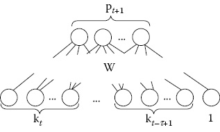
A typical training example in WWW prediction is  〈[kt−τ+1, …, kt−1, kt]T, d〉, where [kt−τ+1, …, kt−1, kt]T is the input to the ANN and d is the target web page. Notice that the input units of the ANN in Figure 3.5 are τ previous pages that the user has recently visited, where k is a web page ID. The output of the network is a Boolean value, not a probability. We will see later how to approximate the probability of the output by fitting a sigmoid function after ANN output. The approximated probabilistic output becomes o′ = f(o(I) = pt+1, where I is an input session and pt+1 = p(d|kt−τ+1, …, kt). We choose the sigmoid function (2.3) as a transfer function so as the ANN can handle nonlinearly separable datasets [MITC97]. Notice that in our ANN design (Figure 3.5), we use a sigmoid transfer function (2.3), in each building block. In Equation 2.3, I is the input to the network, O is the output of the network, W is the matrix of weights, and σ is the sigmoid function:

{o=σ(w.I)σ(y)=11+e −y	(3.3)

E(W)=12∑k∈D∑i∈ouputs(tik−oik)2	(3.4)

{wji=wji+δwjiδwji=−η∂Ed∂w ji	(3.5)

δwji(n)=−η∂Ed∂wji+αδwji(n−1)	(3.6)

We implement the back-propagation algorithm for training the weights. The back-propagation algorithm employs gradient descent to attempt to minimize the squared error between the network output values and the target values of these outputs. The sum of the error over all of the network output units is defined in Equation 3.3. In Equation 3.4, the outputs is the set of output units in the network, D is the training set, and tik and oik are the target and the output values associated with the ith output unit and training example k, respectively. For a specific weight wji in the network, it is updated for each training example as in Equation 2.5, where η is the learning rate and wji is the weight associated with the ith input to the network unit j (for details see [MITC97]). As we can see from Equation 3.5, the search direction δw is computed using the gradient descent that guarantees convergence toward a local minimum. In order to mitigate that, we add a momentum to the weight update rule such that the weight update direction δwji(n) depends partially on the update direction in the previous iteration δwji(n − 1). The new weight update direction is shown in Equation 3.6, where n is the current iterations and α is the momentum constant. Notice that in Equation 3.6, the step size is slightly larger than that in Equation 3.5. This contributes to a smooth convergence of the search in regions where the gradient is unchanging [MITC97].

In our implementation, we set the step size η dynamically based on the distribution of the classes in the dataset. Specifically, we set the step size to large values when updating the training examples that belong to low-distribution classes and vice versa. This is because when the distribution of the classes in the dataset varies widely (e.g., a dataset might have 5% positive examples and 95% negative examples), the network weights converge toward the examples from the class of the larger distribution, which causes a slow convergence. Furthermore, we adjust the learning rates slightly by applying the momentum constant (3.6) to speed up the convergence of the network [MITC97].

3.4 Support Vector Machines

SVM are learning systems that use a hypothesis space of linear functions in a high-dimensional feature space, trained with a learning algorithm from optimization theory. This learning strategy introduced by Vapnik et al. ([VAPN95], [VAPN98], [VAPN95], [CRIS00]) is a very powerful method that has been applied in a wide variety of applications. The basic concept in SVM is the hyper-plane classifier or linear separability. In order to achieve linear separability, SVM applies two basic ideas—margin maximization and kernels, that is, mapping input space to a higher dimension space, feature space.

For binary classification, the SVM problem can be formalized as in Equation 3.7. Suppose we have N training data points {(x1, y1), (x2, y2), …, (xN, yN)}, where xi∈Rd and yi∈{+1, −1}. We would like to find a linear separating hyper-plane classifier as in Equation 3.8. Furthermore, we want this hyper-plane to have the maximum separating margin with respect to the two classes (see Figure 3.6). The functional margin, or the margin for short, is defined geometrically as the Euclidean distance of the closest point from the decision boundary to the input space. Figure 3.7 gives an intuitive explanation of why margin maximization gives the best solution of separation. In Figure 3.7a, we can find an infinite number of separators for a specific dataset. There is no specific or clear reason to favor one separator over another. In Figure 3.7b, we see that maximizing the margin provides only one thick separator. Such a solution proves to achieve the best generalization accuracy, that is, prediction for the unseen ([VAPN95], [VAPN98], [VAPN99]):

{minimize(w,b)12wTwsubjecttoyi(w⋅xi−b)≥1	(3.7)

f(x)=sign(w⋅x−b)	(3.8)

maximizeL(w,b,α)=12wTw−∑i=1Nαiyi(w⋅xi−b)+∑i=1Nαi	(3.9)

f(x)=sign(wx−b)=sign(∑i=1Nαiyi(x⋅xi−b))	(3.10)

Notice that Equation 3.8 computes the sign of the functional margin of point x in addition to the prediction label of x, that is, the functional margin of x equals wx − b.

The SVM optimization problem is a convex quadratic programming problem (in w, b) in a convex set (Equation 3.7). We can solve the Wolfe dual instead (as in Equation 3.9) with respect to α, subject to the constraints that the gradient of L(w, b, α) with respect to the primal variables w and b vanish and αi ≥ 0. The primal variables are eliminated from L(w, b, α) (see [CRIS00] for more details). When we solve αi, we can obtain w=∑i=1Nαiyixi, and we can classify a new object x using Equation 3.10. Note that the training vectors occur only in the form of the dot product and that there is a Lagrangian multiplier αi for each training point, which reflects the importance of the data point. When the maximal margin hyper-plane is found, only points that lie closest to the hyper-plane will have αi > 0, and these points are called support vectors. All other points will have αi = 0 (see Figure 3.8a). This means that only those points that lie closest to the hyper-plane give the representation of the hypothesis/classifier. These most important data points serve as support vectors. Their values can also be used to give an independent boundary with regard to the reliability of the hypothesis/classifier [BART99].

Figure 3.8a shows two classes and their boundaries, that is, margins. The support vectors are represented by solid objects, while the empty objects are nonsupport vectors. Notice that the margins are only affected by the support vectors, that is, if we remove or add empty objects, the margins will not change. Meanwhile any change in the solid objects, either adding or removing objects, could change the margins. Figure 3.8b shows the effects of adding objects in the margin area. As we can see, adding or removing objects far from the margins, for example, data point 1 or −2, does not change the margins. However, adding and/or removing objects near the margins, for example, data point 2 and/or −1, has created new margins.

3.5 Markov Model

Some recent and advanced predictive methods for web surfing are developed using Markov models ([YANG01], [PIRO96]). For these predictive models, the sequences of web pages visited by surfers are typically considered as Markov chains that are then fed as input. The basic concept of the Markov model is that it predicts the next action depending on the result of previous action or actions. Actions can mean different things for different applications. For the purpose of illustration, we will consider actions specific for the WWW prediction application. In WWW prediction, the next action corresponds to the prediction of the next page to be traversed. The previous actions correspond to the previous web pages to be considered. Based on the number of previous actions considered, Markov models can have different orders:

pr(Pk)=pr(Sk)	(3.11)

pr(P2|P1)=pr(S2=P2|S1=P1)	(3.12)

pr(PN|PN−1,…,PN−k)=pr(SN=PN|SN−1=PN−1,…,SN−k=PN−k)	(3.13)

The 0th-order Markov model is the unconditional probability of the state (or web page) (Equation 3.11). In Equation 3.11, Pk is a web page and Sk is the corresponding state. The first-order Markov model, Equation 3.12, can be computed by taking page-to-page transitional probabilities or the n-gram probabilities of {P1, P2}, {P2, P3}, …, {Pk−1, Pk}.

In the following, we present an illustrative example of different orders of the Markov model and how it can predict.

Example:

Imagine a website of six web pages: P1, P2, P3, P4, P5, and P6. Suppose we have user sessions as given in Table 3.1. This table depicts the navigation of many users of that website. Figure 3.9 shows the first-order Markov model, where the next action is predicted based on only the last action performed, that is, the last page traversed by the user. States S and F correspond to the initial and final states, respectively. The probability of each transition is estimated by the ratio of the number of times the sequence of states was traversed and the number of times the anchor state was visited. Next, to each arch in Figure 3.8, the first number is the frequency of that transition, and the second number is the transition probability. For example, the transition probability of the transition (P2 to P3) is 0.2 because the number of times users traverse from page 2 to page 3 is 3 and the number of times page 2 is visited is 15 (i.e., 0.2 = 3/15).

Notice that the transition probability is used to resolve prediction. For example, given that a user has already visited P2, the most probable page he or she visits next is P6. That is because the transition probability from P2 to P6 is the highest.

Notice that the transition probability might not be available for some pages. For example, the transition probability from P2 to P5 is not available because no user has visited P5 after P2. Hence, these transition probabilities are set to zeros. Similarly, the Kth-order Markov model is where the prediction is computed after considering the last Kth action performed by the users (Equation 3.13). In WWW prediction, the Kth-order Markov model is the probability of user visits to PKth page given its previous k − 1 page visits.

Figure 3.10 shows the second-order Markov model that corresponds to Table 3.1. In the second-order model, we consider the last two pages. The transition probability is computed in a similar fashion. For example, the transition probability of the transition (P1, P2) to (P2, P6) is 0.16 = 1 × 1/6 because the number of times users traverse from state (P1, P2) to state (P2, P6) is 1 and the number of times pages (P1, P2) is visited is 6 (i.e., 0.16 = 1/6). The transition probability is used for prediction. For example, given that a user has visited P1 and P2, he or she most probably visits P4 because the transition probability from state (P1, P2) to state (P2, P4) is greater than that from state (P1, P2) to state (P2, P6).

The order of the Markov model is related to the sliding window. The Kth-order Markov model corresponds to a sliding window of size K − 1.

Notice that there is another concept that is similar to the sliding window concept, which is the number of hops. In this appendix, we use the number of hops and the sliding window interchangeably.

In WWW prediction, Markov models are built based on the concept of n-gram. The n-gram can be represented as a tuple of the form 〈x1, x2, …, xn〉 to depict sequences of page clicks by a population of users surfing a website. Each component of the n-gram takes a specific page ID value that reflects the surfing path of a specific user surfing a webpage. For example, the n-gram 〈P10, P21, P4, P12〉 for some user U states that the user U has visited the pages 10, 21, 4, and finally 12 in a sequence.

3.6 Association Rule Mining (ARM)

Association rule mining is a data mining technique that has been applied successfully to discover related transactions. ARM finds the relationships among itemsets based on their co-occurrence in the transactions. Specifically, ARM discovers the frequent patterns (regularities) among those itemsets. For example, what are the items purchased together in a super store? In the following, we briefly introduce ARM. For more details, see [AGRA93] and [AGRA94].

Assume that we have m items in our database; then, define I = {i1, i2, …, im} as the set of all items. A transaction T is a set of items such that T⊆I. Let D be the set of all transactions in the database. A transaction T contains X if X⊆T and X⊆I. An association rule is an implication of the form X→Y, where, X⊂I, Y⊂I, and X∩Y = ϕ. There are two parameters to consider a rule: confidence and support. A rule R = X→Y holds with confidence c if c% of the transactions of D that contain X also contain Y (i.e., c = pr(Y|X)). The rule R holds with support s if s% of the transactions in D contain X and Y (i.e., s = pr(X, Y)). The problem of mining association rules is defined as follows. Given a set of transactions D, we would like to generate all rules that satisfy a confidence and a support greater than a minimum confidence (σ), minconf, and minimum support (ϑ), minsup. There are several efficient algorithms proposed to find association rules such as AIS algorithm ([AGRA93], [AGRA94]), SETM algorithm [HOUT95], and AprioriTid [LIU99].

In the case of web transactions, we use association rules to discover navigational patterns among users. This would help to cache a page in advance and reduce the loading time of a page. Also, discovering a pattern of navigation helps in personalization. Transactions are captured from the clickstream data captured in web server logs.

In many applications, there is one main problem in using ARM, that is, using global minimum support (minsup). This is because rare hits, that is, web pages that are rarely visited, will not be included in the frequent sets because it will not achieve enough support. One solution to this problem is to have a very small support threshold; however, we will end up with very large frequent itemsets, which is computationally hard to handle. Liu et al. [LIU99] proposed a mining technique that uses different support thresholds for different items. Specifying multiple thresholds allow rare transactions that might be very important to be included in the frequent itemsets. Other issues might arise depending on the application itself. For example, in the case of WWW prediction, a session is recorded for each user. The session might have tens of clickstreams (and sometimes hundreds depending on the duration of the session). Using each session as a transaction will not work because it is rare to find two sessions that are frequently repeated (i.e., identical); hence, it will not achieve even a very high support threshold, minsup. There is a need to break each session into many subsequences. One common method for this is to use a sliding window of size w. For example, suppose we use a sliding window w = 3 to break the session S = 〈A, B, C, D, E, E, F〉; then, we will end up with having the subsequences S′ = {〈A, B, C〉, 〈B, C, D〉, 〈C, D, E〉, 〈D, E, F〉}. The total number of subsequences of a session S using window w is length(S)-w. To predict the next page in an active user session, we use a sliding window of the active session and ignore the previous pages. For example, if the current session is 〈A, B, C〉, and the user refer to page D, then the new active session becomes 〈B, C, D〉, using a sliding window 3. Notice that page A is dropped, and 〈B, C, D〉 will be used for prediction. The rationale behind this is because most users go back and forth while surfing the web trying to find the desired information, and it may be most appropriate to use the recent portions of the user history to generate recommendations/predictions [MOBA01].

Mobasher et al. [MOBA01] proposed a recommendation engine that matches an active user session with the frequent itemsets in the database and predicts the next page the user most probably visits. The engine works as follows. Given an active session of size w, the engine finds all the frequent itemsets of length w + 1, satisfying some minimum support minsup and containing the current active session. Prediction for the active session A is based on the confidence (ψ) of the corresponding association rule. The confidence (ψ) of an association rule X→z is defined as ψ(X→z) = σ(X∪z)/σ(X), where the length of z is 1, page p is recommended/predicted for an active session A, iff

The engine uses a cyclic graph called the frequent itemset graph. The graph is an extension of the lexicographic tree used in the tree projection algorithm of Agrawal et al. [AGRA01]. The graph is organized in levels. The nodes in level l has itemsets of size of l. For example, the sizes of the nodes (i.e., the size of the itemsets corresponding to these nodes) in levels 1 and 2 are 1 and 2, respectively. The root of the graph, level 0, is an empty node corresponding to an empty itemset. A node X in level l is linked to a node Y in level l + 1 if X⊂Y. To further explain the process, suppose we have the following sample web transactions involving pages 1, 2, 3, 4, and 5 as given in Table 3.2. The Apriori algorithm produces the itemsets as given in Table 3.3, using a minsup = 0.49. The frequent itemset graph is shown in Figure 3.11.

Suppose we are using a sliding window of size 2, and the current active session A = 〈2,3〉. To predict/recommend the next page, in the frequent itemset graph, we first start at level 2 and extract all the itemsets at level 3 linked to A. From Figure 3.11, the node {2, 3} is linked to {1, 2, 3} and {2, 3, 5} nodes with confidence:

The recommended page is 1 because its confidence is larger. Notice that, in recommendation engines, the order of the clickstream is not considered, that is, there is no distinction between the sessions 〈1, 2, 4〉 and 〈1, 4, 2〉. This is a disadvantage of such systems because the order of pages visited might bear important information about the navigation patterns of users.

3.7 Multiclass Problem

Most classification techniques solve the binary classification problem. Binary classifiers are accumulated to generalize for the multiclass problem. There are two basic schemes for this generalization, namely, one-VS-one and one-VS-all. To avoid redundancy, we will present this generalization only for SVM.

One-VS-one: The one-VS-one approach creates a classifier for each pair of classes. The training set for each pair classifier (i, j) includes only those instances that belong to either class i or j. A new instance x belongs to the class upon which most pair classifiers agree. The prediction decision is quoted from the majority vote technique. There are n(n − 1)/2 classifiers to be computed, where n is the number of classes in the dataset. It is evident that the disadvantage of this scheme is that we need to generate a large number of classifiers, especially if there are a large number of classes in the training set. For example, if we have a training set of 1000 classes, we need 499,500 classifiers. On the other hand, the size of the training set for each classifier is small because we exclude all instances that do not belong to that pair of classes.

One-VS-all: The one-VS-all approach creates a classifier for each class in the dataset. The training set is preprocessed such that for a classifier j instances that belong to class j are marked as class (+1) and instances that do not belong to class j are marked as class (−1). In the one-VS-all scheme, we compute n classifiers, where n is the number of pages that users have visited (at the end of each session). A new instance x is predicted by assigning it to the class that its classifier outputs the largest positive value (i.e., maximal marginal) as in Equation 3.15. We can compute the margin of point x as in Equation 3.13. Notice that the recommended/predicted page is the sign of the margin value of that page (see Equation 3.10):

f(x)=wx−b=∑iNαiyi(x.xi−b)	(3.14)

prediction(x)=argmax1≤c≤Mfc(x)	(3.15)

In Equation 3.15, M is the number of classes, x = 〈x1, x2, …, xn〉 is the user session, and fi is the classifier that separates class i from the rest of the classes. The prediction decision in Equation 3.15 resolves to the classifier fc that is the most distant from the testing example x. This might be explained as fc has the most separating power, among all other classifiers, of separating x from the rest of the classes.

The advantage of this scheme (one-VS-all) compared to the one-VS-one scheme is that it has fewer classifiers. On the other hand, the size of the training set is larger for a one-VS-all scheme than that for a one-VS-one scheme because we use the whole original training set to compute each classifier.

3.8 Image Mining

3.8.1 Overview

While image mining is not directly applicable to the work discussed in this book, we expect big data to include large images and video data. This will also include geospatial data. Therefore, an understanding of image mining is useful so that one can adapt the techniques for image-based big data. More details of our work on image mining including geospatial data can be found in [AWAD09] and [LI07].

Along with the development of digital images and computer storage technologies, a huge amount of digital images are generated and saved every day. Applications of digital image have rapidly penetrated many domains and markets, including commercial and news media photo libraries, scientific and nonphotographic image databases, and medical image databases. As a consequence, we face a daunting problem of organizing and accessing these huge amounts of available images. An efficient image retrieval system is highly desired to find images of specific entities from a database. The system expected can manage a huge collection of images efficiently, respond to users’ queries with high speed, and deliver a minimum of irrelevant information (high precision), as well as ensure that relevant information is not overlooked (high recall).

To generate such kinds of systems, people tried many different approaches. In the early 1990s, because of the emergence of large image collections, content-based image retrieval (CBIR) was proposed. CBIR computes relevance based on the similarity of visual content/low-level image features such as color histograms, textures, shapes, and spatial layout. However, the problem is that visual similarity is not semantic similarity. There is a gap between low-level visual features and semantic meanings. The so-called semantic gap is the major problem that needs to be solved for most CBIR approaches. For example, a CBIR system may answer a query request for a “red ball” with an image of a “red rose.” If we undertake the annotation of images with keywords, a typical way to publish an image data repository is to create a keyword-based query interface addressed to an image database. If all images came with a detailed and accurate description, image retrieval would be convenient based on current powerful pure text search techniques. These search techniques would retrieve the images if their descriptions/annotations contained some combination of the keywords specified by the user. However, the major problem is that most of images are not annotated. It is a laborious, error-prone, and subjective process to manually annotate a large collection of images. Many images contain the desired semantic information, even though they do not contain the user-specified keywords. Furthermore, keyword-based search is useful especially to a user who knows what keywords are used to index the images and who can therefore easily formulate queries. This approach is problematic; however, when the user does not have a clear goal in mind, does not know what is in the database, and does not know what kinds of semantic concepts are involved in the domain.

Image mining is a more challenging research problem than retrieving relevant images in CBIR systems. The goal of image mining is to find an image pattern that is significant for a given set of images and helpful to understand the relationships between high-level semantic concepts/descriptions and low-level visual features. Our focus is on aspects such as feature selection and image classification. It should be noted that image mining and analytics are important for social media as the members of postnumerous images. These images could be used to embed messages that could penetrate into computing systems. Images in social media could also be analyzed to extract various demographics such as location.

3.8.2 Feature Selection

Usually, data saved in databases with well-defined semantics is structured data such as numbers or structured data entries. In comparison, data with ill-defined semantics is unstructured data. Images, audio, and video are data with ill-defined semantics. In the domain of image processing, images are represented by derived data or features such as color, texture, and shape. Many of these features have multi values (e.g., color histogram, moment description) When people generate these derived data or features, they generally generate as many features as possible, since they are not aware which feature is more relevant. Therefore, the dimensionality of derived image data is usually very high. Actually, some of the selected features might be duplicated or may not even be relevant to the problem. Including irrelevant or duplicated information is referred to as noise. Such problems are referred to as the “curse of dimensionality.” Feature selection is the research topic for finding an optimal subset of features. In this chapter, we will discuss this curse and feature selection in detail.

We developed a wrapper-based simultaneous feature weighing and clustering algorithm. Clustering algorithm will bundle similar image segments together and generate a finite set of visual symbols (i.e., blob-token). Based on histogram analysis and chi-square value, we assign features of image segments different weights instead of removing some of them. Feature weight evaluation is wrapped in a clustering algorithm. In each iteration of the algorithm, feature weights of image segments are re-evaluated based on the clustering result. The re-evaluated feature weights will affect the clustering results in the next iteration.

3.8.3 Automatic Image Annotation

Automatic image annotation is research concerned with object recognition, where the effort is concerned with trying to recognize objects in an image and generate descriptions for the image according to semantics of the objects. If it is possible to produce accurate and complete semantic descriptions for an image, we can store descriptions in an image database. Based on a textual description, more functionality (e.g., browse, search, and query) of an image database system could be easily and efficiently implemented by applying many existing text-based search techniques. Unfortunately, the automatic image annotation problem has not been solved in general, and perhaps this problem is impossible to solve.

However, in certain subdomains, it is still possible to obtain some interesting results. Many statistical models have been published for image annotation. Some of these models took feature dimensionality into account and applied singular value decomposition (SVD) or principle component analysis (PCA) to reduce dimension. But none of them considered feature selection or feature weight. We proposed a new framework for image annotation based on a translation model (TM). In our approach, we applied our weighted feature selection algorithm and embedded it in an image annotation framework. Our weighted feature selection algorithm improves the quality of visual tokens and generates better image annotations.

3.8.4 Image Classification

Image classification is an important area, especially in the medical domain because it helps manage large medical image databases and has great potential on diagnostic aid in a real-world clinical setting. We describe our experiments for the image CLEF medical image retrieval task. Sizes of classes of CLEF medical image dataset are not balanced, which is really a serious problem for all classification algorithms. To solve this problem, we resample data by generating subwindows. K nearest neighbor (KNN) algorithm, distance weighted KNN, fuzzy KNN, nearest prototype classifier, and evidence theory-based KNN are implemented and studied. Results show that evidence-based KNN has the best performance based on classification accuracy.

3.9 Summary

In this chapter, we first provided an overview of the various data mining tasks and techniques, and then discussed some of the techniques that we have used in our work. These include neural networks, SVM, and ARM. We have utilized a combination of these techniques together with some other techniques in the literature as well as our own techniques to develop data analytics techniques for very large databases. Some of these techniques are discussed in Parts II through V.

Numerous data mining techniques have been designed and developed, and many of them are being utilized in commercial tools. Several of these techniques are variations of some of the basic classification, clustering, and ARM techniques. One of the major challenges today is to determine the appropriate technique for various applications. We still need more benchmarks and performance studies. In addition, the techniques should result in fewer false positives and negatives. While there is still much to be done, the progress over the last decade has been extremely promising. Our challenge is to develop data mining techniques for big data systems.

References

[AGRA93]. R. Agrawal, T. Imielinski, A. Swami, “Mining Association Rules between Sets of Items in Large Database,” Proceedings of the ACM SIGMOD Conference on Management of Data, Washington, D.C., May, pp. 207–216, 1993.

[AGRA94]. R. Agrawal and R. Srikant, “Fast Algorithms for Mining Association Rules in Large Database,” Proceedings of the 20th International Conference on Very Large Data Bases, San Francisco, CA, pp. 487–499, 1994.

[AGRA01]. R. Agrawal, C. Aggarawal, V. Prasad, “A Tree Projection Algorithm for Generation of Frequent Itemsets,” Journal of Parallel and Distributed Computing Archive 61 (3), 350–371, 2001.

[AWAD09]. M. Awad, L. Khan, B. Thuraisingham, L. Wang, Design and Implementation of Data Mining Tools. CRC Press, Boca Raton, FL, 2009.

[BART99]. P. Bartlett and J. Shawe-Taylor, “Generalization Performance of Support Vector Machines and Other Pattern Classifiers,” Advances in Kernel Methods—Support Vector Learning, B. Schölkopf, C. J. C. Burges, A. J. Smola (eds.), MIT Press, Cambridge, MA, pp. 43–53, 1999.

[CRIS00]. N. Cristianini and J. Shawe-Taylor, Introduction to Support Vector Machines, 1st ed. Cambridge University Press, Cambridge, pp. 93–122, 2000.

[HOUT95]. M. Houtsma and A. Swanu, “Set-Oriented Mining of Association Rules in Relational Databases,” Proceedings of the 11th International Conference on Data Engineering, Washington, D.C., pp. 25–33, 1995.

[LI07]. C. Li, L. Khan, B. M. Thuraisingham, M. Husain, S. Chen, F. Qiu, “Geospatial Data Mining for National Security: Land Cover Classification and Semantic Grouping,” In ISI’07: Proceedings of the IEEE Conference on Intelligence and Security Informatics, May 23−24, New Brunswick, NJ, 2007.

[LIU99]. B. Liu, W. Hsu, Y. Ma, “Mining Association Rules with Multiple Minimum Supports,” Proceedings of the 5th ACM SIGKDD International Conference on Knowledge Discovery and Data Mining, San Diego, CA, pp. 337–341, 1999.

[MITC97]. T. M. Mitchell, Machine Learning. McGraw Hill, New York, NY, Chapter 3, 1997.

[MOBA01]. B. Mobasher, H. Dai, T. Luo, M. Nakagawa, “Effective Personalization Based on Association Rule Discovery from Web Usage Data,” In WIDM01: Proceedings of the ACM Workshop on Web Information and Data Management, pp. 9–15, 2001.

[PIRO96]. P. Pirolli, J. Pitkow, R. Rao, “Silk from a Sow’s Ear: Extracting Usable Structures from the Web,” In CHI-96: Proceedings of the 1996 Conference on Human Factors in Computing Systems, Vancouver, British Columbia, Canada, pp. 118–125, 1996.

[THUR16]. B. Thuraisingham, S. Abrol, R. Heatherly, M. Kantarcioglu, V. Khadilkar, L. Khan, Analyzing and Securing Social Networks. CRC Press, Boca Raton, FL, 2016.

[VAPN95]. V. N. Vapnik, The Nature of Statistical Learning Theory. Springer, New York, NY, 1995.

[VAPN98]. V. N. Vapnik, Statistical Learning Theory. Wiley, New York, 1998.

[VAPN99]. V. N. Vapnik, The Nature of Statistical Learning Theory. Springer-Verlag, Berlin, 1999.

[YANG01]. Q. Yang, H. Zhang, T. Li, “Mining Web Logs for Prediction Models in WWW Caching and Prefetching,” The 7th ACM SIGKDD International Conference on Knowledge Discovery and Data Mining, Aug. 26–29, pp. 473–478, 2001.