
Chapter 5. Programming R with RStudio
Programming R involves the writing, editing, debugging, and documenting of functions; working with function files; and packaging functions for wider distribution. In this chapter we look at some components of RStudio that simplify these and other tasks.
Source Code Editor
Recall that RStudio leverages numerous web technologies. A major one is the Ace code editor (ace.ajax.org) for editing functions and files. Ace is written in JavaScript, which allows all necessary computations to be done in the client, thereby avoiding numerous calls to the server. This is important, as an editor for an IDE must do many things well and quickly, such as:
File-type specific syntax highlighting
Automatic code indentation
Parenthesis matching
Working with many documents simultaneously
Working with large documents
Working with different languages
While not as feature-rich as some editors—say, the Emacs editor that powers ESS—the Ace editor in the RStudio framework is still quite able and easy to work with. The component uses tabs to organize the files and provides toolbars and other means to issue common commands quickly.
Basics
The action to open a new file in the Source code editor is presented in many
different ways: under the File >
New menu item, the leftmost toolbar button in the
application-wide toolbar pops up the choices, and the keyboard shortcut
opens an R file. The code editor can open text files of various types.
The menu items include an R Script, a
Text File, an Sweave Document, and a TeX Document. In Figure 5-1, we show how the component’s
toolbar adjusts to provide file-type specific actions.
Similarly, existing files can be opened through a menu item, a
toolbar button or a keyboard shortcut. In addition, active links in the
Files browser can be used to open a
file. A selection of recently opened files is available through the
application toolbar and the menu.

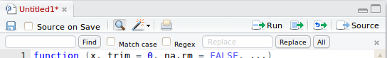
Files that have unsaved changes are marked with an asterisk next
to their name in their tab’s label. For such files, the standard
Save and Save as… actions are also accessed through the
menu bar, the application-wide toolbar, or keyboard shortcuts. In
addition, the Save with Encoding…
menu item can be used to specify an encoding for the file when saving.
As a convenience, the Save All action
is available through the menu bar or application-wide toolbar.
A file can be closed by clicking on the “x” icon in the tab for a file, through a menu item, or through the appropriate keyboard shortcut, Ctrl+W or Cmd+W. (Except for the Chrome browser under Mac OS X, where Ctrl+Shift+L is used, as the other shortcut is used to close the browser window.) If there are unsaved changes, you will be asked whether you want to save the work.
The editor allows one to have many different files open at once.
When a moderate-sized number of files are open, one navigates between
them by clicking on the appropriate tab. There are shortcuts for cycling
through the tabs (Next, Previous, First, Last). As well, the widget provides a means to
select a tab to jump to. This is especially useful if there are so many
tabs that their labels don’t fit in the allocated width (Figure 5-2). This widget provides a drop-down menu and
a search box.

The Find and Replace menu item
implements a search through the currently opened file. When run through
a web browser, the browser’s search function may search through the
entire page. There is no such feature in the desktop version.
(Therefore, each component has its own search bar.)
Instead of a search dialog, the Ace editor produces an unobtrusive
pop-down bar in the code editor (Figure 5-3)
that allows a user to find (and replace) strings of text. Checkboxes
allow one to restrict the search by case-matching or widen it using
regular expressions (see ?regex). The Find button marches through the document
moving to each new match, wrapping at the end of the document. The
Replace and All buttons control how to replace the found
text with an alternative.
The Editing pane of the Options
dialog (Figure 3-4) has
options for adjusting the behavior of the editor. In that screenshot,
you can see we have turned off the automatic insertion of matching
parentheses and quotes, but otherwise the defaults are to our particular
taste.
There is also an option to toggle line numbering. When this option is on, line numbers appear along the left margin. In either case, down in the lower left corner of the code-editor window is a label (Figure 5-5) listing the current line number and position of the cursor.
File synchronization
When a file is opened in the editor, it is not locked and may be modified through some other process, such as being altered by your favorite editor. RStudio will monitor changes in the underlying file and propagate them back.
Keyboard shortcuts
In Table 5-1, we list several keyboard shortcuts provided by RStudio for basic editing needs. There are the standard operating system shortcuts for things like cut, copy, and paste; undo and redo, etc. In addition, some, such as the “yank” commands, come from the Emacs world.
| Action | Windows and Linux | Mac OS X |
Undo | Command+Z | |
Redo | Ctrl+Shift+Z | Command+Shift+Z |
Cut | Ctrl+X | Command+X |
Copy | Ctrl+C | Command+C |
Paste | Ctrl+V | Command+V |
Select All | Ctrl+A | Command+A |
Jump to Word | Ctrl+Left/Right | Option+Left/Right |
Jump to Start/End | Ctrl+Home/End or Ctrl+Up/Down | Command+Home/End or Command+Up/Down |
Delete Line | Ctrl+D | Command+D |
Select | Shift+[Arrow] | Shift+[Arrow] |
Select Word | Ctrl+Shift+Left/Right | Option+Shift+Left/Right |
Select to Line Start | Shift+Home | Command+Shift+Left or Shift+Home |
Select to Line End | Shift+End | Command+Shift+Right or Shift+End |
Select Page Up/Down | Shift+PageUp/PageDown | Shift+PageUp/Down |
Select to Start/End | Ctrl+Shift+Home/End or Shift+Alt+Up/Down | Command+Shift+Up/Down |
Delete Word Left | Ctrl+Backspace | Option+Backspace or Ctrl+Option+Backspace |
Delete Word Right | n/a | Option+Delete |
Delete to Line End | n/a | Ctrl+K |
Delete to Line Start | n/a | Option+Backspace |
Indent | Tab (at beginning of line) | Tab (at beginning of line) |
Outdent | Shift+Tab | Shift+Tab |
Yank line up to cursor | Ctrl+U | Ctrl+U |
Yank line after cursor | Ctrl+K | Ctrl+K |
Insert currently yanked text | Ctrl+Y | Ctrl+Y |
Insert assignment operator | Alt+- | Option+- |
R Programming Features
RStudio augments the Ace editor with some R-specific conveniences.
Syntax highlighting
Syntax highlighting is implemented by RStudio for files related to R development (Figure 5-4). Highlighting provides separate colors for keywords, functions, and other objects, so they are readily identified. There isn’t much for the R programmer to do here except enjoy the benefits.

Having comments in a different color from the text makes them
much more readable and at the same time unobtrusive. Working with
comments in R involves simply placing a pound (#) symbol somewhere on a line, so that the
text to the right is ignored by the interpreter. (There are no
Emacs-like comment conventions for repeated pound symbols.) Comments
can be added to an entire block of text through the Comment/Uncomment Lines menu item (under the
magic wand). Simply select the text, and this action will toggle the
comment state.
Bracket matching
The R syntax requires several matching delimiters, such as matching square brackets for vector extraction, matching parentheses for functions, matching braces for blocks of commands, and matching quotes for strings. RStudio has two means to assist the bookkeeping required for this demand. It can be done either automatically through the insertion of a matching bracket when the opening one is given—or if this is turned off, through highlighting. A setting in the Editing pane of the Options dialog is used to adjust the behavior.
Automatic indenting
Within code blocks delimited by curly braces, it can be useful
to have indenting to quickly identify the level of nesting. This is
quite common—for instance, a simple for loop within a function body has this
nesting. RStudio automatically indents the next line after the Enter
key is pressed. In addition, pressing the Tab key when the cursor is
at the start of a line will indent that line.
For indenting the current line or formatting a selected region, the magic wand has the action “Reindent Lines” (also Ctrl+I ).
Code completion and usage information
The Tab key completion features of the console (see Tab Completion) are also present when working with the code editor. To review, a token is the last word or fragment in a given line. When the Tab key is pressed, the completions for this token and its context are analyzed:
- Object completion
When the token is a partially typed object name, the candidates for completion include objects available in the global workspace. If possible, the completion provides a summary for each candidate from R’s help mechanism.
- Argument completion
When the token is the opening of a function, the candidates include a list and a description of the function’s arguments from the function’s help page.
- Argument or object completion
When the token is at a function argument and a start is given, the completion includes matching argument names and matching objects, as either could be given.
- String completion
Candidates for string completion are the filenames in the current working directory.
Extract function
In our case study, we took on the task of converting a script of
commands into a package, creating several functions in the process.
The Extract Function feature (the
magic wand toolbar button) helps facilitate this, trying to create a
function from the currently selected lines in an R script. To use this
feature, highlight the commands that you want to include in the
definition of the function, then invoke the magic wand. A dialog
gathers a function name, then the selected commands are parsed to make
a guess as to what the argument to the function should be.
Run or source commands
We mentioned in R Script Files that one can select parts of an R script in the code editor and send the commands to the R interpreter. The Ctrl+Enter and Ctrl+Shift+Enter shortcuts make this process very convenient (the full list was provided in Table 3-2).
Navigation
As projects grow, it is typical to have multiple files, each containing many functions grouped in some manner. Being able to navigate quickly within a file and among files becomes a welcome convenience.
Jump to function
In addition to searching through a file, RStudio has features for navigating among the functions in an R script file. The “Jump to function” action is invoked through a menu item, a keyboard shortcut (Ctrl-Alt-Up), or a pop up located in the bottom status bar of the code editor window (Figure 5-5). Selecting a function moves the cursor to the beginning of the function’s definition.

Go to file/function
To quickly navigate between files and functions within a
project, RStudio provides the tremendously useful Go to File/Function action with the shortcut
Ctrl+. . The application’s tool bar always shows
this, and the shortcut moves the focus to this entry area. This action
provides a text entry box where a user can type either a function name
or file name. Automatic completion candidates are given from both, so
one can quickly and conveniently jump around within a project. The
files and functions that make up a project are monitored for changes,
so even changes external to RStudio can be tracked.
The File Browser
The Files browser (Figure 5-6) displays the files and subdirectories
of a given directory. The refresh toolbar button will refresh this
display, if clicked. There are just a few actions. Clicking on a
subdirectory will load the contents of that directory into the file
browser. Clicking on a file will open an editor or viewer for that file.
For text files with certain extensions, this will be the source-code
editor. Otherwise, this will be a system program if the source-code
editor is not appropriate. For example, a .pdf file
will open in a PDF viewer on the desktop; or from the browser (server
version), in a new window; whereas a .doc file will
open in Microsoft Word (or the associated program for the MIME type) on
the desktop, but will be downloaded when run from the browser.

By selecting one or more files through the checkboxes on the left,
one can initiate actions to delete, rename, copy, or move the file(s)
through actions available from the toolbar buttons. One can create new
folders through the New Folder
toolbar button. If these actions are not sufficient, in the desktop
version, the More > Show Folder In New
Window toolbar item will invoke the system file manager for
the directory.
File upload
For server usage, there is a toolbar button to initiate a file upload. This is similar to attaching a file to an email, a reasonable analogy, as you may also be restricted from uploading files that are too large.
Debugging R Code in RStudio
R provides some useful tools for debugging R code, summarized online at http://www.stats.uwo.ca/faculty/murdoch/software/debuggingR/debug.shtml. These tools allow R users to investigate errors, step through functions, insert debugging code, etc. Although RStudio currently doesn’t have additional integration with R’s debugging tools, the RStudio console does work with these functions.
Package Maintenance
R uses packages to extend itself and RStudio
provides the Packages browser to make
it effortless to load, install, update, and/or delete packages in the
library of packages.
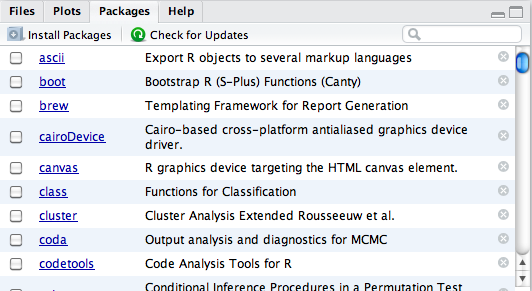
In Figure 5-7 we show a screenshot. Each
installed package is shown with a description derived from the package’s
DESCRIPTION file. In addition, for each
package there is:
A checkbox to load (
require) or unload (detach) the packageAn active link to open the help page index of the package
A delete icon to uninstall the package from the library
The Packages browser toolbar has
a Check for Updates button, which is
used to see if any packages have pending updates. The dialog this opens is
similar to Figure 5-8, where those
packages with possible updates on a system are listed. One simply selects
the packages to update and then presses the Install Updates button. From there, RStudio
calls install.packages to download the
new packages from a repository to install.

You can install new packages through the dialog that opens when you
press the Install
Packages toolbar button (Figure 5-9). In
the figure, the “Install dependencies” checkbox is selected, instructing
install.packages to also download and
install any packages that the desired ones depend on. In addition, several
other things must be specified:
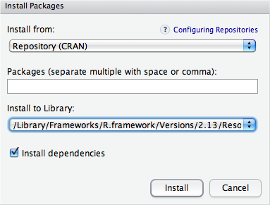
- Which package
Which package (or packages) to install is specified in the middle text entry box titled “Packages”. There are over 3,000 packages, so presenting them all in a list is a poor interface. Rather than browsing through the available choices, the text entry box has an auto-completion feature that shows available packages matching the currently typed text token.
- Which repository
Packages are hosted on
CRANand elsewhere.CRANis a system of repositories that mirror a central repository in Austria. One must choose a specific one from which to download the files. RStudio will keep track of this choice. If this has not been done, a dialog to choose a CRAN mirror will appear before the Install Packages dialog. One may also choose to install from a local “Package Archive File.” The help-page link for “Configuring Repositories” shows the manual page forsetRepositories, which spells out how one specifies non-CRAN repositories, such as those for the BioConductor project.- Which directory
R will look for installed packages in several places (e.g., system-wide locations and user-specific locations) but won’t scan the entire hard drive. When installing a package, one must specify which places will be checked. The dialog provides a combobox to select a Library directory. The available choices are determined by consulting the
.libPathsfunction. This function both returns the places where packages are looked for and allows one to append to this search list. The server version allows a choice of a directory in the user’s home directory, as otherwise certain permissions would be required. For the desktop version, if a local, user-only spot is desired, one can call the.libPathsfunction from the console to provide the desired location.
Organizing Activities with Projects
RStudio allows one to organize their work and files into projects, with each project having its own associated directory and global workspace. This is a fantastic feature for keeping your different workflows separate. Projects can also take advantage of RStudio’s version control features (Version Control with RStudio), giving you confidence that you can recover from erroneous changes and easily collaborate with others.
When a project is opened, much of the past session is restored. The project’s profile, data and history files are restored, the working directory is reset, the previously opened files are reopened, and RStudio’s layout settings are set to match when the project was last closed.
The upper-right corner of the main application toolbar holds the
project selector. This shows the currently selected project (if any)—and
more importantly, provides a convenient way to to create a new project,
switch to a different project, close the current project, or adjust
options for the current project. These actions are also found under the
Project menu where there is also the additional option
to open a project in a new window. This is used to open more than one
project simultaneously. To select a project, one browses for the
proj file created with the project.
Creating a new project is straightforward. The wizard for doing so first asks (Figure 5-10) if you want to start with a new directory, use a new directory, or check out a project which is using version control. Selecting the new directory option requires (Figure 5-11) that one specifies a name, a directory and indicate if version control is to be used.
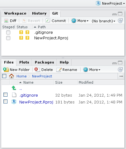
Figure 5-12 shows how after creating a new
project with a Git repository, the tabbed Git pane
appears, as well as some new files are created in the project’s
directory.
While one is working within a project, any changes to the workspace
are stored with the project (unless this behavior is changed through the
Project Options dialog). The files in the directory are
indexed to look for changes, allowing the “Go to file/function” search box
to be used to quickly navigate to any defined function in the
project.


Version Control with RStudio
RStudio’s project infrastructure allows a project to be integrated in with one of two popular version control systems, Git and Subversion. Both are widely used: e.g., the R project uses Subversion, whereas RStudio uses Git. Version control systems provide two very useful features:
They keep a history of changes to a file and allow one to browse or rollback to previous versions. This is similar to what is provided by Apple Computer’s popular Time Machine software for backups.
Version control systems allow multiple users to work on the same project without stepping on each other’s toes. This is similar to how the Track Changes feature of Microsoft Word allows groups to work collaboratively on a Word document, but better, as changes can be made by all parties at the same time and the version control system merges the changes together. This only requires intervention when there are conflicts.
Getting started with version control
RStudio makes the cost of using version control so minimal that it is highly recommended for any new project. Before getting started, you must have the underlying version control tools installed on your system: one of the open-source projects, Git or Subversion. We will focus on Git in the following section.
If Git is not installed, the main Git website (http://www.git-scm.com/) points to downloads for both Windows and Mac OS X users and a source download for Linux users, if the underlying distribution doesn’t provide a pre-compiled solution. Installation is typically straightforward. If needed, more details on installation (along with much more not touched on here) are given in the Git Community Book, http://book.git-scm.com/.
Using Git to keep a history of changes
When a project is under version control, then that software will
track changes to the files in its repository. There are different
possible file states as compared to those recognized in the
repository: a file can not be in the repository, the file can have
been deleted from the repository, a file can be deleted locally but
still in the repository, or the file can be modified from that in the
repository. RStudio tracks these differences and displays them in its
Git pane. In Figure 5-12,
there are two new files on the file system that are not in the
repository. In Figure 5-13, we illustrate how the
Git pane and the Files pane
account for files in a different manner, depending on their state.
This information is equivalent to the command git status.

The Staged column in the
Git pane has checkboxes that instruct Git to index
that file to be included in the repository during the next commit,
providing the functionality of the command git add.
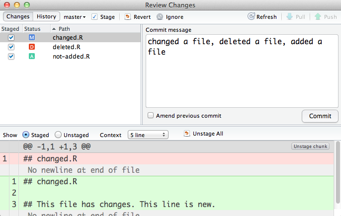
Putting staged changes into the repository is called
“committing.” The Commit icon in the
Git panes toolbar opens the Review
Changes dialog to assist with this task. In Figure 5-14, we show the dialog for committing three
changes. In the upper-right corner of the dialog is an area to leave a
message associated with the commit. Though leaving a message is
technically optional, one should strive to give short but informative
messages, as they are very helpful when auditing file changes.
Selecting the History view in the dialog shows
previously left messages (along with much more).
In the top-left corner of the dialog appears a list of the files that differ from the repository. Again, one can adjust whether a file is staged or not. The currently selected file has its differences between the repository and the file system highlighted, allowing a quick review of what is new.
If you change your mind on a commit, you can check out an old
copy of the file. The Git command git
checkout allows this. This isn’t directly provided by the
interface. However, RStudio provides a convenient way to issue
arbitrary Git commands through a built-in Git shell. The shell is
raised through the menu item More >
Shell.... The command git checkout HEAD^
deleted.R would then check out the file that was deleted and
allow you to stage it for reinclusion.
Git allows one to make “branches” of a project that can be
reintegrated back into the main project. This is a convenient way to
experiment with changes without worrying about the impact on the
current project along the way. To make a branch, the Git command
git branch branch_name is used. RStudio makes it
trivial to choose among the current branches, as next to the refresh
icon in the Git pane’s toolbar is a selector to
switch between branches. In Figure 5-15, we show the
History view after creating a branch and adding a
new file experimental.R to it. This file is in
the new branch but not the old. To merge a branch back into the
master, the git merge branch_name command is used.

Collaborating with Git
One of the great features of Git is the ability to collaborate
with others on a project. There are two concepts: we “pull” changes
made by others, and we “push” our changes back to others. When we
check out a project from a Git repository, RStudio activates these
options in the Review Changes dialog. Figure 5-16 shows the output of clicking
Pull after our local copy of a repository requested
updates made on the repository hosted at www.github.com, an enormously popular
hosting site for Git projects. When connecting to such sites, it may
be necessary to authenticate, typically through SSH. RStudio includes
the necessary platform files to make this work similarly on all
platforms.

When collaborating, there is always the possibility that you or
your colleagues may be working on the same thing. In particular, you
may both have made changes to the same file. While resolving different
edits is often possible without intervention, this is not always the
case. When it is not, the merge command of Git
reports back to RStudio the actions that need to be taken. In Figure 5-17, we see such a report.

Case Study: Report Generation using Sweave
In two previous case studies, we saw how RStudio can be used in an interactive manner, and how RStudio can be used to write the functions that compose a package. In this example, we look at how RStudio can be used to write reports where we automatically mix R output into the report. If our data changes, we just rerun it. This allows us to keep all our numbers and references in sync. It allows us to create reproducible research, as the document contains all the code needed to produce it. The main tool is Sweave, a literate programming tool for R that can “weave” R commands into a document, formatted with marked-up text. (Typically, but not necessarily, this is LaTeX, which we illustrate here—but there are other implementations for Open Office, asciidoc, etc.)
Knitr
The knitr package is a newer alternative to Sweave.
A vignette is a longer form of documentation for R packages and is
usually written using Sweave. For our naked mole rat package, we have
provided our colleagues with functions and documented them using roxygen2. Now we see how to write a vignette,
allowing us to mix in our observations and insights along with use cases
and detail about the functionality we have provided.
Vignettes can simply be a Sweave file saved in the inst/doc subdirectory of the package. When a package is “checked,” the vignette’s code is executed; when a package is “built,” a pdf file is created for distribution with the package. There is some control over this—for more detail, see the section Writing Package Vignettes in the Writing R Extensions manual.
To begin, we open a file nmr.Rnw after creating
the doc directory through the Files browser. RStudio’s code-editor File > New menu has an option for a new
Sweave Document, which we select. The code-editor
toolbar and status bar are specific to the document type. For an
Sweave document, which mixes R code and
LaTex markup, it makes sense to allow the user to run
commands in the console, so that option is still present. There is also a
new Compile PDF button, which, when
clicked, initiates the process of calling Sweave to replace the R commands with their
output in a new file (the “weaving”) and then calls R’s texi2dvi function to create a
pdf file. (This all assumes a working
LaTeX is installed on your machine. If
LaTeX is installed but a warning appears, its path
may need to be specified.)
Figure 5-18 shows the code editor opened to
a vignette. The lower-right corner indicates that it is editing an
Sweave Document, and syntax
highlighting is present both for the R code and the
LaTeX text.

LaTeX is a markup language (the lingua franca of mathematicians) too complicated to describe here, but certainly not impossible to learn. It really helps to start with a basic template, such as this (LaTeX uses the percent sign for a comment character):
documentclass[12pt]{article}       %% A declaration of type
usepackage{geometry}               %% A LaTeX package
%
%VignetteIndexEntry{Using the NMRpackage} %% Meta data lines
%VignettePackage{NMRpackage}
%VignetteDepends{zoo}
%
	itle{NMRpackage}                  %% A LaTeX macro call
author{John Verzani}
%
egin{document}                    %% Latex is between begin/end document
maketitle                          %% Call a macro to make title
%
% ... Insert text here ...
%
end{document}                      %% End the document
The template shows how LaTeX calls commands
(maketitle) and uses begin/end
environment pairs to mark larger sections of text.
The integration of R with LaTeX is done in two ways:
- Code chunks
Code chunks are one or more commands to be executed, wrapped within tags beginning with
<<>>=and ending with@. Within the<<>>, one can place directives to adjust what happens:With no directives, the code is echoed back with the output interspersed
To name a block of code, the first directive should be a name (other arguments are in the form
key=value). When named, this output can then be referred to through<<name>>To suppress the code being echoed back, use
echo=FALSE.To suppress the code being evaluated, use
eval=FALSE.To suppress the results being included, use
results=hide.To have LaTeX process the output (as opposed to having it included verbatim), use
results=tex.To include a figure in the code, use
fig=TRUE. Forlatticegraphics, one also needs to callprinton the graph object.
- Inline code
An R session inline; the expression can refer to variables defined in previous chunks.
For example, the following text would create a new section and a graphic:
section{Making a plot}
The package provides the 	exttt{nmrTsPlot} function to make a time series
graph using the 	exttt{ggplot2} package. For example,
<<nmrTsPlot, fig=TRUE>>=
f <- system.file("sampledata","degas.txt", package="NMRpackage")
a <- readNMRData(f)
b <- createZooObjects(a)
m <- createStateMatrix(b)
out <- nmrTsPlot(m[, 1:4])
print(out)
@
Tables are straightforward, but can be tedious to typeset in
LaTeX. Conveniently, one can use R to convert a
rectangular object (matrix or data frame) to a table, using the add-on
xtable package.
In the following we make a matrix, d, that holds the number of times that mole
i is in the same chamber as mole
j, by looping over the rows of the state matrix using
apply. Then we use xtable to create the table. The echo=FALSE argument suppresses the R code, and
results=tex is used to indicate that
this output should be processed as LaTeX code:
<<makeTable, echo=FALSE>>=
n <- 8
d <- matrix(integer(n^2), nrow=n)
ind <- combn(1:n, 2)
f <- function(r) {
  apply(ind, 2, function(ij) {
    i <- ij[1]; j <- ij[2]
    x <- r[i] == r[j]
    if(!is.na(x))
      d[j,i] <<- d[i,j] <<- d[i, j] + as.numeric(x)
  })
}

out <- apply(m[, 1:n], 1, f)
diag(d) <- "-"
@

<<echo=FALSE, results=tex>>=
require(xtable)
out <- xtable(d, caption="Number of events mole rat $i$ is in same chamber as mole rat $j$")
print(out)
@
To create a pdf file from our vignette, we click the Compile PDF toolbar button. This calls the
compilePdf function provided by RStudio
(which delegates to texi2dvi from the
tools package). (Or, if using
devtools, the build_vignettes function is available.) RStudio
can also process plain LaTeX files; the process is
identical. If the file extension matches one of the common extensions for
weaving (Rnw, Snw,
nw), Sweave is called first, then texidvi.
When an Rnw file is compiled, R first produces a tex file with the R commands interspersed, then LaTeX is run on this file. Doing so creates a number of files including a pdf file containing the output (if successful), a log file listing warnings and errors (if present), and perhaps others (e.g., an aux file). Most of these may be safely deleted, as they will be regenerated if needed.
If successful, the pdf file can be opened in a
native viewer, or one can click on its link in the Files browser. If unsuccessful, one peruses the
console output or the log file to find the
errors.