Conceived by Burton Howard Bloom in 1970, a Bloom filter is a probabilistic data structure used to test whether a member is an element of a set. Bloom filters have a strong space advantage over other data structures such as a Java Set, in that each element uses the same amount of space, no matter its actual size. For example, a string of 32 characters takes up the same amount of memory in a Bloom filter as a string of 1024 characters, which is drastically different than other data structures. Bloom filters are introduced as part of a pattern in Bloom Filtering.

While the data structure itself has vast memory advantages, it is not always 100% accurate. While false positives are possible, false negatives are not. This means the result of each test is either a definitive “no” or “maybe.” You will never get a definitive “yes.” With a traditional Bloom filter, elements can be added to the set, but not removed. There are a number of Bloom filter implementations that address this limitation, such as a Counting Bloom Filter, but they typically require more memory. As more elements are added to the set, the probability of false positives increases. Bloom filters cannot be resized like other data structures. Once they have been sized and trained, they cannot be reverse-engineered to achieve the original set nor resized and still maintain the same data set representation.

The following variables are used in the more detailed explanation of a Bloom filter below:

A Bloom filter is represented by a continuous string of m bits initialized to zero. For each element in n, k hash function values are taken modulo m to achieve an index from zero to m - 1. The bits of the Bloom filter at the resulting indices are set to one. This operation is often called training a Bloom filter. As elements are added to the Bloom filter, some bits may already be set to one from previous elements in the set. When testing whether a member is an element of the set, the same hash functions are used to check the bits of the array. If a single bit of all the hashes is set to zero, the test returns “no.” If all the bits are turned on, the test returns “maybe.” If the member was used to train the filter, the k hashs would have set all the bits to one.

The result of the test cannot be a definitive “yes” because the bits may have been turned on by a combination of other elements. If the test returns “maybe” but should have been “no,” this is known as a false positive. Thankfully, the false positive rate can be controlled if n is known ahead of time, or at least an approximation of n.

The following sections describe a number of common use cases for Bloom filters, the limitations of Bloom filters and a means to tweak your Bloom filter to get the lowest false positive rate. A code example of training and using a Hadoop Bloom filter can be found in Bloom filter training.

This section lists a number of common use cases for Bloom filters. In any application that can benefit from a Boolean test prior to some sort of expensive operation, a Bloom filter can most likely be utilized to reduce a large number of unneeded operations.

The false positive rate is the largest downside to using a Bloom filter. Even with a Bloom filter large enough to have a 1% false positive rate, if you have ten million tests that should result in a negative result, then about a hundred thousand of those tests are going to return positive results. Whether or not this is a real issue depends largely on the use case.

Traditionally, you cannot remove elements from a Bloom filter set after training the elements. Removing an element would require bits to be set to zero, but it is extremely likely that more than one element hashed to a particular bit. Setting it to zero would destroy any future tests of other elements. One way around this limitation is called a Counting Bloom Filter, which keeps an integer at each index of the array. When training a Bloom filter, instead of setting a bit to zero, the integers are increased by one. When an element is removed, the integer is decreased by one. This requires much more memory than using a string of bits, and also lends itself to having overflow errors with large data sets. That is, adding one to the maximum allowed integer will result in a negative value (or zero, if using unsigned integers) and cause problems when executing tests over the filter and removing elements.

When using a Bloom filter in a distributed application like MapReduce, it is difficult to actively train a Bloom filter in the sense of a database. After a Bloom filter is trained and serialized to HDFS, it can easily be read and used by other applications. However, further training of the Bloom filter would require expensive I/O operations, whether it be sending messages to every other process using the Bloom filter or implementing some sort of locking mechanism. At this point, an external database might as well be used.

Before training a Bloom filter with the elements of a set, it can be very beneficial to know an approximation of the number of elements. If you know this ahead of time, a Bloom filter can be sized appropriately to have a hand-picked false positive rate. The lower the false positive rate, the more bits required for the Bloom filter’s array. Figure A-1 shows how to calculate the size of a Bloom filter with an optimal-k.

Figure A-1. Optimal size of a Bloom filter with an optimal-k

The following Java helper function calculates the optimal m.

/**
 * Gets the optimal Bloom filter sized based on the input parameters and the
 * optimal number of hash functions.
 *
 * @param numElements
 *            The number of elements used to train the set.
 * @param falsePosRate
 *            The desired false positive rate.
 * @return The optimal Bloom filter size.
 */
public static int getOptimalBloomFilterSize(int numElements,
        float falsePosRate) {
    return (int) (-numElements * (float) Math.log(falsePosRate)
                / Math.pow(Math.log(2), 2));
}

The optimal-k is defined as the number of hash functions that should be used for the Bloom filter. With a Hadoop Bloom filter implementation, the size of the Bloom filter and the number of hash functions to use are given when the object is constructed. Using the previous formula to find the appropriate size of the Bloom filter assumes the optimal-k is used.

Figure A-2 shows how the optimal-k is based solely on the size of the Bloom filter and the number of elements used to train the filter.

Figure A-2. Optimal-k of a Bloom filter

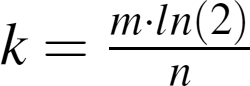
The following helper function calculates the optimal-k.

/**
 * Gets the optimal-k value based on the input parameters.
 *
 * @param numElements
 *            The number of elements used to train the set.
 * @param vectorSize
 *            The size of the Bloom filter.
 * @return The optimal-k value, rounded to the closest integer.
 */
public static int getOptimalK(float numElements, float vectorSize) {
    return (int) Math.round(vectorSize * Math.log(2) / numElements);
}