![]()
Data Types and Advanced Data Types
Transact-SQL is a strongly-typed language. Columns and variables must have a valid data type, and the type is a constraint of the column. In this chapter, we will not cover all data types comprehensively. We will skip the obvious part and concentrate on specific information and on more complex and sophisticated data types that were introduced in SQL Server over time.
Basic Data Types
Basic data types like integer or varchar are pretty much self-explanatory. Some of these types have interesting and important-to-know properties or behavior, and even the most used, like varchar, are worth a look.
Many tools, like the Microsoft Access Upsizing Wizard, generate tables in SQL Server using some default choices. For all character strings, they create nvarchar columns by default. The n stands for UNICODE, the double-bytes representation of a character, with enough room to fit all worldwide language signs (also called logograms in liguistics), like traditional and simplified Chinese, Arabic, and Farsi. nvarchar must be used when the column has to store non-European languages, but as they induce an obvious overhead, you should avoid creating unneeded nvarchar or nchar columns.
The real size of the data in bytes is returned by the DATALENGTH() function, while the LEN() string function, designed to hide internal storage specifics from the T-SQL developer, will return the number of characters. We test the different values returned by these functions in Listing 10-1. The results are shown in Figure 10-1.
Listing 10-1. Unicode Handling
DECLARE
    @string VARCHAR(50) = 'hello earth',
    @nstring NVARCHAR(50) = 'hello earth';

SELECT
    DATALENGTH(@string) as DatalengthString,
    DATALENGTH(@nstring) as DatalengthNString,
    LEN(@string) as lenString,
    LEN(@nstring) as lenNString;

Figure 10-1. The Results of LEN() and DATALENGTH()
You can see the the nvarchar storage of our 'hello earth' is 22 bytes. Imagine a 100 million-row table: having such a column with an average of 11-character strings, the storage needed to accomodate the extra bytes would be 1.1 GB.
![]() Note To represent a T-SQL identifier, like a login name or a table name, you can use the special sysname type, which corresponds to nvarchar(128).
Note To represent a T-SQL identifier, like a login name or a table name, you can use the special sysname type, which corresponds to nvarchar(128).
The Max Data Types
In the heady days of SQL Server 2000, large object (LOB) data storage and manipulation required use of the old style text, ntext, and image data types. These types have been deprecated and were replaced with easier-to-use types in SQL Server 2005, namely the varchar(max), nvarchar(max), and varbinary(max) types.
Like the older types, each of these new data types can hold over 2.1 billion bytes of character or binary data, but they handle data in a much more efficient way. The old text or image types required a dedicated type of allocation that created a b-tree structure for each value inserted, regardless of its size. This of course had a significant performance impact when retrieving the columns’ content, because the storage engine had to follow pointers to this complex allocation structure for each and every row being read, even if its value was a few bytes long. The (n)varchar(max) or varbinary(max) are more clever types that are handled differently depending on the size of the value. The storage engine creates the LOB structure only if the data inserted cannot be kept in the 8 KB page.
Also, unlike the legacy LOB types, the max data types operate similarly to the standard varchar, nvarchar, and varbinary data types. Standard string manipulation functions such as LEN() and CHARINDEX(), which didn’t work well with the older LOB data types, work as expected with the new max data types. The new data types also eliminate the need for awkward solutions involving the TEXTPTR, READTEXT, and WRITETEXT statements to manipulate LOB data.
![]() Note The varchar(max), nvarchar(max), and varbinary(max) data types are complete replacements for the SQL Server 2000 text, ntext, and image data types. The text, ntext, and image data types and their support functions will be removed in a future version of SQL Server. Because they are deprecated, Microsoft recommends you avoid these older data types for new development.
Note The varchar(max), nvarchar(max), and varbinary(max) data types are complete replacements for the SQL Server 2000 text, ntext, and image data types. The text, ntext, and image data types and their support functions will be removed in a future version of SQL Server. Because they are deprecated, Microsoft recommends you avoid these older data types for new development.
The new max data types support a .WRITE clause extension to the UPDATE statement to perform optimized minimally logged updates and appends to varchar(max), varbinary(max), and nvarchar(max) types. You can use the .WRITE clause by appending it to the end of the column name in your UPDATE statement. The example in Listing 10-2 compares performance of the .WRITE clause to a simple string concatenation when updating a column. The results of this simple comparison are shown in Figure 10-2.
Listing 10-2. Comparison of .WRITE Clause and String Append
-- Turn off messages that can affect performance
SET NOCOUNT ON;
-- Create and initially populate a test table
CREATE TABLE #test (
    Id int NOT NULL PRIMARY KEY,
    String varchar(max) NOT NULL
);

INSERT INTO #test (
    Id,
    String
) VALUES (
    1,
    ''
), (
    2,
    ''
);
-- Initialize variables and get start time
DECLARE @i int = 1;
DECLARE @quote varchar(50) = 'Four score and seven years ago...';
DECLARE @start_time datetime2(7) = SYSDATETIME();
-- Loop 2500 times and use .WRITE to append to a varchar(max) column
WHILE @i < 2500
BEGIN
    UPDATE #test
    SET string.WRITE(@quote, LEN(string), LEN(@quote))
    WHERE Id = 1;

    SET @i += 1;
END;

SELECT '.WRITE Clause', DATEDIFF(ms, @start_time, SYSDATETIME()), 'ms';

-- Reset variables and get new start time
SET @i  = 1;
SET @start_time = SYSDATETIME();

-- Loop 2500 times and use string append to a varchar(max) column
WHILE @i < 2500
BEGIN
    UPDATE #test
    SET string += @quote
    WHERE Id = 2;

    SET @i += 1;
END;

SELECT 'Append Method', DATEDIFF(ms, @start_time, SYSDATETIME()), 'ms';

SELECT
    Id,
    String,
    LEN(String)
FROM #test;

DROP TABLE #test;

Figure 10-2. Testing the .WRITE Clause against Simple String Concatenation
As you can see in this example, the .WRITE clause is appreciably more efficient than a simple string concatenation when updating a max data type column. Note that these times were achieved on one of our development machines, and your results may vary significantly depending on your specific configuration. You can expect the .WRITE method to perform more efficiently than simple string concatenation when updating max data type columns, however.
You should note the following about the .WRITE clause:
- The second .WRITE parameter, @offset, is a zero-based bigint and cannot be negative. The first character of the target string is at offset 0.
- If the @offset parameter is NULL, the expression is appended to the end of the target string. @length is ignored in this case.
- If the third parameter, @length, is NULL, SQL Server truncates anything past the end of the string expression (the first .WRITE parameter) after the target string is updated. The @length parameter is a bigint and cannot be negative.
There are two types of numeric: exact and approximate. Integer and decimal are exact numbers. It is worth knowing that any exact numeric can be used as an auto-incremented IDENTITY column. Most of the time of course, a 32-bit int is chosen as an auto-incremented surrogate key.
![]() Note We call surrogate key a technical, non-natural unique key, in other words a column storing values created inside the database, and having no meaning outside of it. Most of the time in SQL Server it is an IDENTITY (auto-incremented) number, of a uniqueidentifier (a Globally Unique Identifier, or GUID) that we will see later in this chapter.
Note We call surrogate key a technical, non-natural unique key, in other words a column storing values created inside the database, and having no meaning outside of it. Most of the time in SQL Server it is an IDENTITY (auto-incremented) number, of a uniqueidentifier (a Globally Unique Identifier, or GUID) that we will see later in this chapter.
Because there is no unsigned numeric in SQL Server, the range of values that can be generated by the IDENTITY property is from −2,147,483,648 to +2,147,483,647. Indeed, as the IDENTITY property takes a seed and an increment as parameters, nothing prevents you from declaring it as in Listing 10-3:
Listing 10-3. Use the Full Range of 32-bit Integer for IDENTITY Columns
CREATE TABLE dbo.bigtable (
    bigtableId int identity(-2147483648,1) NOT NULL
);

INSERT INTO dbo.bigtable DEFAULT VALUES;
INSERT INTO dbo.bigtable DEFAULT VALUES;

SELECT * FROM dbo.bigtable;
The seed parameter of the bigtableId column IDENTITY property is set as the lowest possible int value, instead of the most commonly seen IDENTITY(1,1) declaration. The results follow in Figure 10-3.

Figure 10-3. The First Two IDENTITY Values Inserted
This allows for twice the range of available values in your key and might save you from choosing a bigint (64-bit integer) to accommodate values for a table in which you expect to have more than 2 billion rows but less than 4 billion rows. Once again, on a 100-million row table, it will save about 400 MB, and probably much more than that because there are strong chances that the key value will be used in indexes and foreign keys.
![]() Note Some are reluctant to use this tip because it creates keys with negative numbers. Theoretically, a surrogate key is precisely meaningless by nature and should not be seen by the end user. It is merely there to provide a unique value to identify and reference a row. Sometimes, when these surrogate keys are shown to users, they start to acquire a life of their own, a purpose. For example, people start to talk about customer 3425 instead of using her name—hence the difficulty with negative values.
Note Some are reluctant to use this tip because it creates keys with negative numbers. Theoretically, a surrogate key is precisely meaningless by nature and should not be seen by the end user. It is merely there to provide a unique value to identify and reference a row. Sometimes, when these surrogate keys are shown to users, they start to acquire a life of their own, a purpose. For example, people start to talk about customer 3425 instead of using her name—hence the difficulty with negative values.
We talked about exact numeric types. A word of caution about approximate type: do not use approximate numeric types for anything other than scientific purpose. A column defined as float or real stores floating-point values as defined by the IEEE Standard for Floating-Point Arithmetic (IEEE 754), and any result of an operation on float or real will be approximate. Think about the number pi: you always give a non-precise representation of pi, and you will never get the precise value of pi because you need to round or truncate it at some decimal. To store the precise decimal values that most of us manipulate in business applications—amounts, measurements, etc.— you need to use either money or decimal which are fixed data types.
The bit data type is mostly used to store Boolean values. It can be 0, 1, or NULL, and it consumes one byte of storage, but with an optimization: if you create up to 8-bit columns in your table, they will share the same byte. So bit columns take very little space. SQL Server recognizes also the string values 'TRUE' and 'FALSE' when they are applied to a bit, and they will be converted to 1 and 0, respectively.
The date and time types were enriched in SQL Server 2008 by the distinct date and time types, and the more precise datetime2 and datetimeoffset. Before that, only datetime and smalldatetime were available. Table 10-1 summarizes the differences between all SQL Server 2014 date and time data types before we delve more into details.
Table 10-1. SQL Server 2012 Date and Time Data Type Comparison

The date data type allows solving a very common problem we had until SQL server 2008. How can we express date without having to take time into account? Before date, it was tricky to do a straight comparison as shown in Listing 10-4.
Listing 10-4. Date Comparison
SELECT *
FROM Person.StateProvince
WHERE ModifiedDate = '2008-03-11';
Because the ModifiedDate column data type is datetime, SQL Server converts implictly the '2008-03-11' value to the full '2008-03-11 00:00:00.000' datetime representation before carrying out the comparison. If the ModifiedDate time part is not '00:00:00.000', no line will be returned, which is the case in our example. With datetime-like data types, we are forced to do things as shown in Listing 10-5.
Listing 10-5. Date Comparison Executed Correctly
SELECT *
FROM Person.StateProvince
WHERE ModifiedDate BETWEEN '2008-03-11' AND '2008-03-12';
-- or
SELECT *
FROM Person.StateProvince
WHERE CONVERT(CHAR(10), ModifiedDate, 126) = '2008-03-11';
But both tricks are unsatisfactory. The first one has a flaw: because the BETWEEN operator is inclusive, lines with ModifiedDate set at '2008-03-12 00:00:00.000' would be included. To be safe, we should have written the query as in Listing 10-6.
Listing 10-6. Correcting the Date Comparison
SELECT *
FROM Production.Product
WHERE ModifiedDate BETWEEN '2008-03-11' AND '2008-03-11 23:59:59.997';
-- or
SELECT *
FROM Person.StateProvince
WHERE ModifiedDate >= '2008-03-11' AND ModifiedDate < '2008-03-12';
The second example, in Listing 10-5, has a performance implication, because it makes the condition non-sargable.
![]() Note We say that a predicate is sargable (from Search ARGument–able) when it can take advantage of an index seek. Here, no index on the ModifiedDate column can be used for a seek operation if its value is altered in the query, and thus does not match what was indexed in the first place.
Note We say that a predicate is sargable (from Search ARGument–able) when it can take advantage of an index seek. Here, no index on the ModifiedDate column can be used for a seek operation if its value is altered in the query, and thus does not match what was indexed in the first place.
So, the best choice we had was to enforce, maybe by trigger, that every value entered in the column had its time part stripped off or written with '00:00:00.000', but that time part was still taking up storage space for nothing. Now, the date type, costing 3 bytes, stores a date with one day accuracy.
Listing 10-7 shows a simple usage of the date data type, demonstrating that the DATEDIFF() function works with the date type just as it does with the datetime data type.
Listing 10-7. Sample Date Data Type Usage
-- August 19, 14 C.E.
DECLARE @d1 date = '0014-08-19';

-- February 26, 1983
DECLARE @d2 date = '1983-02-26';
SELECT @d1  AS Date1, @d2 AS Date2, DATEDIFF(YEAR, @d1,  @d2) AS YearsDifference;
The results of this simple example are shown in Figure 10-4.

Figure 10-4. The Results of the Date Data Type Example
In contrast to the date data type, the time data type lets you store time-only data. The range for the time data type is defined on a 24-hour clock, from 00:00:00.0000000 through 23:59:59.9999999, with a user-definable fractional second precision of up to seven digits. The default precision, if you don’t specify one, is seven digits of fractional second precision. Listing 10-8 demonstrates the time data type in action.
Listing 10-8. Demonstrating Time Data Type Usage
-- 6:25:19.1 AM
DECLARE @start_time time(1) = '06:25:19.1'; -- 1 digit fractional precision
-- 6:25:19.1234567 PM
DECLARE @end_time time = '18:25:19.1234567'; -- default fractional precision
SELECT @start_time AS start_time, @end_time AS end_time,
DATEADD(HOUR, 6, @start_time) AS StartTimePlus, DATEDIFF(HOUR, @start_time, @end_time) AS
 EndStartDiff;
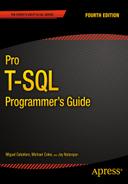
In Listing 10-8, two data type instances are created. The @start_time variable is explicitly declared with a fractional second precision of one digit. You can specify a fractional second precision of one to seven digits with 100-nanosecond (ns) accuracy; the fixed fractional precision of the classic datetime data type is three digits with 3.33-millisecond (ms) accuracy. The default fractional precision for the time data type, if no precision is specified, is seven digits. The @end_time variable in the listing is declared with the default precision. As with the date and datetime data types, the DATEDIFF() and DATEADD() functions also work with the time data type. The results of Listing 10-8 are shown in Figure 10-5.
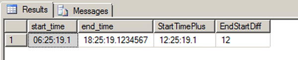
Figure 10-5. The Results of the Time Data Type Example
The cleverly named datetime2 data type is an extension to the standard datetime data type. The datetime2 data type combines the benefits of the date and time data types, giving you the wider date range of the date data type and the greater fractional-second precision of the time data type. Listing 10-9 demonstrates simple declaration and usage of datetime2 variables.
Listing 10-9. Declaring and Querying Datetime2 Variables
DECLARE @start_dt2 datetime2 = '1972-07-06T07:13:28.8230234',
        @end_dt2   datetime2 = '2009-12-14T03:14:13.2349832';
SELECT @start_dt2 AS start_dt2, @end_dt2 AS end_dt2;
The results of Listing 10-9 are shown in Figure 10-6.

Figure 10-6. Declaring and Selecting Datetime2 data Type Variables
The datetimeoffset data type builds on datetime2 by adding the ability to store offsets relative to the International Telecommunication Union (ITU) standard for Coordinated Universal Time (UTC) with your date and time data. When creating a datetimeoffset instance, you can specify an offset that complies with the ISO 8601 standard, which is in turn based on UTC. Basically, the offset must be specified in the range -14:00 to +14:00. The Z offset identifier is shorthand for the offset designated “zulu,” or +00:00. Listing 10-10 shows the datetimeoffset data type in action.
Listing 10-10. Datetimeoffset Data Type Sample
DECLARE @start_dto datetimeoffset = '1492-10-12T13:29:59.9999999-05:00';
SELECT @start_dto AS start_to, DATEPART(YEAR, @start_dto) AS start_year;
The results of Listing 10-10 are shown in Figure 10-7.

Figure 10-7. The Result of the Datetimeoffset Sample
A sampling of possible offsets is shown in Table 10-2. Note that this list is not exhaustive, but demonstrates some common offsets.
Table 10-2. Common Standard Time Zones
|
Time Zone Offset |
Name |
Locations |
|---|---|---|
|
–10:00 |
Hawaii-Aleutian Standard |
Alaska (Aleutian Islands), Hawaii |
|
–08:00 |
Pacific Standard |
US West Coast; Los Angeles, CA |
|
–05:00 |
Eastern Standard |
US East Coast; New York, NY |
|
–04:00 |
Atlantic Standard |
Bermuda |
|
+00:00 |
Coordinated Universal |
Dublin, Lisbon, London |
|
+01:00 |
Central European |
Paris, Berlin, Madrid, Rome |
|
+03:00 |
Baghdad |
Kuwait, Riyadh |
|
+06:00 |
Indian Standard |
India |
|
+09:00 |
Japan Standard |
Japan |
Some people see the acronym UTC and think that it stands for “Universal Time Coordination” or “Universal Time Code.” Unfortunately, the world is not so simple. When the ITU standardized Coordinated Universal Time, it was decided that it should have the same acronym in every language. Of course, international agreement could not be reached, with the English-speaking countries demanding the acronym CUT and French-speaking countries demanding that TUC (temps universel coordonné) be used. In the final compromise, the nonsensical UTC was adopted as the international standard.
You may notice that we use “military time,” or the 24-hour clock, when representing time in the code samples throughout this book. There’s a very good reason for that—the 24-hour clock is an ISO international standard. The ISO 8601 standard indicates that time should be represented in computers using the 24-hour clock to prevent ambiguity.
The 24-hour clock begins at 00:00:00, which is midnight or 12 am. Noon, or 12 pm, is represented as 12:00:00. One second before midnight is 23:59:59, or 11:59:59 pm. In order to convert the 24-hour clock to am/pm time, simply look at the hours. If the hours are less than 12, then the time is am. If the hours are equal to 12, you are in the noon hour, which is pm. If the hours are greater than 12, subtract 12 and add pm to your time.
So, with all these types at your disposal, which do you choose? As a rule, avoid datetime: it doesn’t align with the SQL Standard, takes generally more space and has lower precision than the other types. It costs 8 bytes, ranges from 1753 through 9999, and rounds the time to 3 milliseconds. For example, let’s try the code in Listing 10-11.
Listing 10-11. Demonstration of Datetime Rounding
SELECT CAST('2011-12-31T23:59:59.999' as datetime) as WhatTimeIsIt;
You can see the result in Figure 10-8.
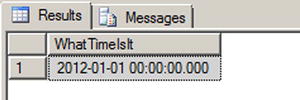
Figure 10-8. The Results of the Datetime Rounding Sample
The 999 milliseconds were rounded to the next value, and 998 would have been rounded to 997. For most usages this is not an issue, but datetime2 does not have this drawback, or at least you have control over it by defining the precision.
One of the difficulties of T-SQL is the handling of dates in the code. Internally, the date and time data types are stored in a numeric representation, but of course, they have to be made human-readable in a string format. The format is important for input or output, but it has nothing to do with storage, and it is a common misconception to consider that a date is stored in a particular format. The output is managed by the client. For example, in SSMS, dates are always returned in the ODBC API ts (timestamp) format (yyyy-mm-dd hh:mm:ss.. . .), regardless of the computer’s regional settings. If you want to force a particular format in T-SQL, you will need to use a conversion function. The CONVERT() function is a legacy function that returns a formatted string from a date and time data type or vice-versa, while the FORMAT() function, introducedin SQL Server 2012, uses the more common .NET format strings and an optional culture to return a formatted nvarchar value. We demonstrate usage of these two functions in Listing 10-12.
Listing 10-12. CONVERT() and FORMAT() Usage Sample
DECLARE @dt2 datetime2 = '2011-12-31T23:59:59';

SELECT FORMAT(@dt2, 'F', 'en-US') as with_format,
        CONVERT(varchar(50), @dt2, 109) as with_convert;
The results are shown in Figure 10-9.

Figure 10-9. The Results of the Datetime2 Formatting Sample
Of course, data input must also be done using a string representation that can be understood by SQL Server as a date. This depends on the language settings of the session. Each session has a language environment that is the default language of the login, unless a SET LANGUAGE command changed it at some time. You can retrieve the language of the current session with one of the two ways shown in Listing 10-13.
Listing 10-13. How to Check the Current Language of the Session
SELECT language
FROM sys.dm_exec_sessions
WHERE session_id = @@SPID;
-- or
SELECT @@LANGUAGE;
Formatting your date strings for input with a language dependent format is risky, because anyone running the code under another language environment would get an error, as shown in Listing 10-14.
Listing 10-14. Language Dependent Date String Representations
DECLARE @lang sysname;

SET @lang = @@LANGUAGE

SELECT CAST('12/31/2012' as datetime2); --this works

SET LANGUAGE 'spanish';

SELECT
    CASE WHEN TRY_CAST('12/31/2012' as datetime2) IS NULL
    THEN 'Cast failed'
    ELSE 'Cast succeeded'
END AS Result;

SET LANGUAGE @lang;
The second CAST() attempt, using the TRY_CAST() to prevent an exception from being raised, will return ‘Cast failed’ because 'MM/dd/yyyy' is not recognized as a valid date format in Spanish. If we would have used CAST() instead of TRY_CAST(), we would have received a conversion error in the Spanish language, and the last SET LANGUAGE command wouldn’t have been executed, due to the preceding exception.
You have two options to prevent this. First, you can use the SET DATEFORMAT instruction that sets the order of the month, day, and year date parts for interpreting date character strings, as shown in Listing 10-15.
Listing 10-15. Usage of SET DATEFORMAT
SET DATEFORMAT mdy;
SET LANGUAGE 'spanish';
SELECT CAST('12/31/2012' as datetime2); --this works now
Or you can decide—this is a better option—to stick with a language-neutral format that will be recognized regardless of what the language environment is. You can do that by making sure you always have your date strings formatted in an ISO 8601 standard variant. In ISO 8601, date and time values are organized from the most to the least significant, starting with the year. The two most common ones are yyyy-MM-ddTHH:mm:ss (note the T character to separate date and time) and yyyyMMdd HH:mm:ss. In a .NET client code, you could generate those formats with the .NET format strings, as shown in the pseudo-code examples of Listing 10-16.
Listing 10-16. Samples of ISO 8601 Date Formatting in .NET Pseudo-code
DateTime.Now.Format( "s" );
DateTime.Now.ToString ( "s", System.Globalization.CultureInfo.InvariantCulture );
The first line calls the Format() method of the the DateTime .NET type, and the second line uses the ToString() method of .NET objects, that can take a format string and a culture as parameters when applied to a DateTime.
With more complete and precise date and time data types comes also a wide range of built-in date- and time-related functions. You might already know the GETDATE() and CURRENT_TIMESTAMP functions. Since SQL Server 2008, you have had more functions for returning the current date and time of the server.
The SYSDATETIME() function returns the system date and time, as reported by the server’s local operating system, as a datetime2 value without time offset information. The value returned by GETDATE(), CURRENT_TIMESTAMP and SYSDATETIME() is the date and time reported by Windows on the computer where your SQL Server instance is installed.
The SYSUTCDATETIME() function returns the system date and time information converted to UTC as a datetime2 value. As with the SYSDATETIME() function, the value returned does not contain additional time offset information.
The SYSDATETIMEOFFSET() function returns the system date and time as a datetimeoffset value, including the time offset information. Listing 10-17 uses these functions to display the current system date and time in various formats. The results are shown in Figure 10-10.
Listing 10-17. Using the Date and Time Functions
SELECT SYSDATETIME() AS [SYSDATETIME];
SELECT SYSUTCDATETIME() AS [SYSUTCDATETIME];
SELECT SYSDATETIMEOFFSET() AS [SYSDATETIMEOFFSET];

Figure 10-10. The Current System Date and Time in a Variety of Formats
The TODATETIMEOFFSET() function allows you to add time offset information to date and time data without time offset information. You can use TODATETIMEOFFSET to add time offset information to a date, time, datetime, datetime2, or datetimeoffset value. The result returned by the function is a datetimeoffset value with time offset information added. Listing 10-18 demonstrates by adding time offset information to a datetime value. The results are shown in Figure 10-11.
Listing 10-18. Adding an Offset to a Datetime Value
DECLARE @current datetime = CURRENT_TIMESTAMP;
SELECT @current AS [No_0ffset];
SELECT TODATETIMEOFFSET(@current, '-04:00') AS [With_0ffset];

Figure 10-11. Converting a Datetime Value to a Datetimeoffset
The SWITCHOFFSET() function adjusts a given datetimeoffset value to another given time offset. This is useful when you need to convert a date and time to another time offset. In Listing 10-19, we use the SWITCHOFFSET() function to convert a datetimeoffset value in Los Angeles to several other regional time offsets. The values are calculated for Daylight Saving Time. The results are shown in Figure 10-12.
Listing 10-19. Converting a Datetimeoffset to Several Time Offsets
DECLARE @current datetimeoffset = '2012-05-04 19:30:00 -07:00';
SELECT 'Los Angeles' AS [Location], @current AS [Current Time]
UNION ALL
SELECT 'New York', SWITCHOFFSET(@current, '-04:00')
UNION ALL
SELECT 'Bermuda', SWITCHOFFSET(@current, '-03:00')
UNION ALL
SELECT 'London', SWITCHOFFSET(@current, '+01:00'),

Figure 10-12. Date and Time Information in Several Different Time Offsets
![]() Tip You can use the Z time offset in datetimeoffset literals as an abbreviation for UTC (+00:00 offset). You cannot, however, specify Z as the time offset parameter with the TODATETIMEOFFSET and SWITCHOFFSET functions.
Tip You can use the Z time offset in datetimeoffset literals as an abbreviation for UTC (+00:00 offset). You cannot, however, specify Z as the time offset parameter with the TODATETIMEOFFSET and SWITCHOFFSET functions.
Time offsets are not the same thing as time zones. A time offset is relatively easy to calculate—it’s simply a plus or minus offset in hours and minutes from the UTC offset (+00:00), as defined by the ISO 8601 standard. A time zone, however, is an identifier for a specific location or region and is defined by regional laws and regulations. Time zones can have very complex sets of rules that include such oddities as Daylight Saving Time (DST). SQL Server uses time offsets in calculations, not time zones. If you want to perform date and time calculations involving actual time zones, you will have to write custom code. Just keep in mind that time zone calculations are fairly involved, especially since calculations like DST can change over time. Case in point—the start and end dates for DST were changed to extend DST in the United States beginning in 2007.
The Uniqueidentifier Data Type
In Windows, you see a lot of GUIDs (Globally Unique IDentifiers) in the registry and as a way to provide code and modules (like COM objects) with unique identifiers. GUIDs are 16-byte values generally represented as 32-character hexadecimal strings, and can be stored in SQL Server in the uniqueidentifier data type. uniqueidentifier could be used to create unique keys across tables, servers or data centers. To create a new GUID and store it in a uniqueidentifier column, you use the NEWID() function, as demonstrated in Listing 10-20. The results are shown in Figure 10-13.
Listing 10-20. Using Uniqueidentifier
CREATE TABLE dbo.Document (
    DocumentId uniqueidentifier NOT NULL PRIMARY KEY DEFAULT (NEWID())
);

INSERT INTO dbo.Document DEFAULT VALUES;
INSERT INTO dbo.Document DEFAULT VALUES;
INSERT INTO dbo.Document DEFAULT VALUES;

SELECT * FROM dbo.Document;
Figure 10-13. Results Generated by the Newid() Function
Each time the NEWID() function is called, it generates a new value using an algorithm based on a pseudo-random generator. The risk of two generated numbers being the same is statistically negligible: hence the global uniqueness it offers.
However, usage of uniqueidentifier columns should be carefully considered, because it bears significant consequences. We have already talked about the importance of data type size, and especially key size. Choosing a uniqueidentifier over an int as a primary key creates an overhead of 12 bytes per row that impacts the size of the table, of the primary key index, of all other indexes if the primary key is defined as clustered (as it is by default), and of all tables that have a foreign key associated to it, and finally on all indexes on these foreign keys. Needless to say, it could considerably increase the size of your database.
There is another problem with uniqueidentifier values, because of their inherent randomness. If your primary key is clustered, the physical order of the table depends upon the value of the key, and at each insert or update, SQL Server must place the new or modified lines at the right place, in the right data pages. GUID random values will cause page splits that will noticeably decrease performances and generate table fragmentation.
To address this last issue, SQL Server 2008 introduced the NEWSEQUENTIALID() function to use as a default constraint with an uniqueidentifier primary key. NEWSEQUENTIALID() generates sequential GUIDs in increasing order. Its usage is shown in Listing 10-21. Results are shown in Figure 10-14; notice that the GUID digits are displayed in groups in reverse order. In the results, the first byte of each GUID represents the sequentially increasing values generated by NEWSEQUENTIALID() with each row inserted.
Listing 10-21. Generating Sequential GUIDs
CREATE TABLE #TestSeqID (
    ID uniqueidentifier DEFAULT NEWSEQUENTIALID() PRIMARY KEY NOT NULL,
    Num int NOT NULL
);

INSERT INTO #TestSeqID (Num)
VALUES (1), (2), (3);

SELECT ID, Num
FROM #TestSeqID;

DROP TABLE #TestSeqID;

Figure 10-14. Results Generated by the NEWSEQUENTIALID Function
The Hierarchyid Data Type
The hierarchyid data type offers a new twist on an old model for representing hierarchical data in the database. This data type introduced in SQL Server 2008 offers built-in support for representing your hierarchical data using one of the simplest models available: materialized paths.
Representing Hierarchical Data
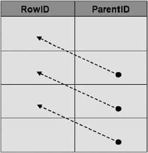
The representation of hierarchical data in relational databases has long been an area of interest for SQL developers. The most common model of representing hierarchical data with SQL Server is the adjacency list model. In this model, each row of a table maintains a reference to its parent row. The following illustration demonstrates how the adjacency list model works in an SQL table.
The AdventureWorks sample database makes use of the adjacency list model in its Production.BillOfMaterials table, where every component references its parent assembly.
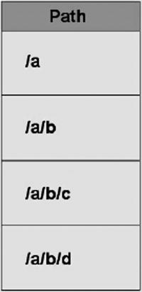
The materialized path model requires that you store the actual hierarchical path from the root node to the current node. The hierarchical path is similar to a modern file system path, where each folder or directory represents a node in the path. The hierarchyid data type supports generation and indexing of materialized paths for hierarchical data modeling. The following illustration shows how the materialized path might look in SQL.
It is a relatively simple matter to represent adjacency list model data using materialized paths, as you’ll see later in this section in the discussion on converting AdventureWorks adjacency list data to the materialized path model using the hierarchyid data type.
Another model for representing hierarchical data is the nested sets model. In this model, every row in the table is considered a set that may contain or be contained by another set. Each row is assigned a pair of numbers defining the lower and upper bounds for the set. The following illustration shows a logical representation of the nested sets model, with the lower and upper bounds for each set shown to the set’s left and right. Notice that the sets in the figure are contained within one another logically, in a structure from which this model derives its name.

In this section, we’ll use the AdventureWorks Production.BillOfMaterials table extensively to demonstrate the adjacency list model, the materialized path model, and the hierarchyid data type. Technically speaking, a bill of materials (BOM), or “parts explosion,” is a directed acyclic graph. A directed acyclic graph is essentially a generalized tree structure in which some subtrees may be shared by different parts of the tree. Think of a cake recipe, represented as a tree, in which “sugar” can be used multiple times (once in the “cake mix” subtree, once in the “frosting” subtree, and so on). This book is not about graph theory, though, so we’ll pass on the technical details and get to the BOM at hand. Although directed acyclic graph is the technical term for a true BOM, we’ll be representing the AdventureWorks BOMs as materialized path hierarchies using the hierarchyid data type, so you’ll see the term hierarchy used a lot in this section.
In order to understand the AdventureWorks BOM hierarchies, it’s important to understand the relationship between product assemblies and components. Basically, a product assembly is composed of one or more components. An assembly can become a component for use in other assemblies, defining the recursive relationship. All components with a product assembly of NULL are top-level components, or “root nodes,” of each hierarchy. If a hierarchyid data type column is declared a primary key, it can contain only a single hierarchyid root node.
The hierarchyid data type stores hierarchy information as an optimized materialized path, which is a very efficient way to store hierarchical information. We will go though a complete example of its use.
Hierarchyid Example
In this example, we will convert the AdventureWorks BOMs to materialized path form using the hierarchyid data type. The first step, shown in Listing 10-22, is to create the table that will contain the hierarchyid BOMs. To differentiate it from the Production.BillOfMaterials table, we have called this table Production.HierBillOfMaterials.
Listing 10-22. Creating the Hierarchyid Bill of Materials Table
CREATE TABLE Production.HierBillOfMaterials
(
    BomNode hierarchyid NOT NULL PRIMARY KEY NONCLUSTERED,
    ProductAssemblyID int NULL,
    ComponentID int NULL,
    UnitMeasureCode nchar(3) NULL,
    PerAssemblyQty decimal(8, 2) NULL,
    BomLevel AS BomNode.GetLevel()
);
The Production.HierBillOfMaterials table consists of the BomNode hierarchyid column, which will contain the hierarchical path information for each component. The ProductAssemblyID, ComponentID, UnitMeasureCode, and PerAssemblyQty are all pulled from the source tables. BomLevel is a calculated column that contains the current level of each BomNode. The next step is to convert the adjacency list BOMs to hierarchyid form, which will be used to populate the Production.HierBillOfMaterials table. This is demonstrated in Listing 10-23.
Listing 10-23. Converting AdventureWorks BOMs to hierarchyid Form
;WITH BomChildren
(
    ProductAssemblyID,
    ComponentID
)
AS
(
    SELECT
        b1.ProductAssemblyID,
        b1.ComponentID
    FROM  Production.BillOfMaterials b1
    GROUP BY
        b1.ProductAssemblyID,
        b1.ComponentID
),
BomPaths
(
    Path,
    ComponentID,
    ProductAssemblyID
)
AS
(
    SELECT
        hierarchyid::GetRoot() AS Path,
        NULL,
        NULL
    UNION ALL

    SELECT
        CAST
        ('/' + CAST (bc.ComponentId AS varchar(30)) + '/' AS hierarchyid) AS Path,
        bc.ComponentID,
        bc.ProductAssemblyID
    FROM BomChildren AS bc
    WHERE bc.ProductAssemblyID IS NULL

    UNION ALL

    SELECT
        CAST
        (bp.path.ToString()  +
            CAST(bc.ComponentID AS varchar(30)) + '/' AS hierarchyid) AS Path,
        bc.ComponentID,
        bc.ProductAssemblyID
    FROM BomChildren AS bc
    INNER JOIN BomPaths AS bp
        ON bc.ProductAssemblyID = bp.ComponentID
)
INSERT INTO Production.HierBillOfMaterials
(
    BomNode,
    ProductAssemblyID,
    ComponentID,
    UnitMeasureCode,
    PerAssemblyQty
)
SELECT
    bp.Path,
    bp.ProductAssemblyID,
    bp.ComponentID,
    bom.UnitMeasureCode,
    bom.PerAssemblyQty
FROM BomPaths AS bp
LEFT OUTER JOIN Production.BillOfMaterials bom
    ON  bp.ComponentID = bom.ComponentID
        AND COALESCE(bp.ProductAssemblyID, -1) = COALESCE(bom.ProductAssemblyID, -1)
WHERE bom.EndDate IS NULL
GROUP BY
    bp.path,
    bp.ProductAssemblyID,
    bp.ComponentID,
    bom.UnitMeasureCode,
    bom.PerAssemblyQty;
This statement is a little more complex than the average hierarchyid data example you’ll probably run into, since most people currently out there are demonstrating conversion of the simple, single-hierarchy AdventureWorks organizational chart. The AdventureWorks Production.BillOfMaterials table actually contains several individual hierarchies.
We will go through the code step by step here to show you exactly what’s going on in this statement. The first part of the statement is a common table expression (CTE) called BomChildren. It returns all ProductAssemblyIDs and ComponentIDs from the Production.BillOfMaterials table.
;WITH BomChildren
(
    ProductAssemblyID,
    ComponentID
)
AS
(
    SELECT
        b1.ProductAssemblyID,
        b1.ComponentID
    FROM Production.BillOfMaterials b1
    GROUP BY
        b1.ProductAssemblyID,
        b1.ComponentID
),
While the organizational chart represents a simple top-down hierarchy with a single root node, the BOM is actually composed of dozens of separate hierarchies with no single hierarchyid root node. BomPaths is a recursive CTE that returns the current hierarchyid, ComponentID, and ProductAssemblyID for each row.
BomPaths
(
    Path,
    ComponentID,
    ProductAssemblyID
)
The anchor query for the CTE is in two parts. The first part returns the root node for the entire hierarchy. In this case, the root just represents a logical grouping of all the BOM’s top-level assemblies; it does not represent another product that can be created by mashing together every product in the AdventureWorks catalog.
SELECT
    hierarchyid::GetRoot(),
    NULL,
    NULL
The second part of the anchor query returns the hierarchyid path to the top-level assemblies. Each top-level assembly has its ComponentId appended to the root path, represented by a leading forward slash (/).
SELECT
    CAST
    ('/'  + CAST (bc.ComponentId AS varchar(30)) + '/' AS hierarchyid) AS Path,
    bc.ComponentID,
    bc.ProductAssemblyID
FROM BomChildren AS bc
WHERE bc.ProductAssemblyID IS NULL
The recursive part of the CTE recursively appends forward slash-separated ComponentId values to the path to represent each component in any given assembly:
    SELECT
        CAST
        (bp.path.ToString()  +
            CAST(bc.ComponentID AS varchar(30)) + '/' AS hierarchyid) AS Path,
        bc.ComponentID,
        bc.ProductAssemblyID
    FROM BomChildren AS bc
    INNER JOIN BomPaths AS bp
        ON bc.ProductAssemblyID = bp.ComponentID
)
The next part of the statement inserts the results of the recursive BomPaths CTE into the Production.HierBillOfMaterials table. The results of the recursive CTE are joined to the Production.BillOfMaterials table for a couple of reasons:
- to ensure that only components currently in use are put into the hierarchy by making sure that the EndDate is NULL for each component
- to retrieve the UnitMeasureCode and PerAssemblyQty columns for each component
We use a LEFT OUTER JOIN in this statement instead of an INNER JOIN because of the inclusion of the hierarchyid root node, which has no matching row in the Production.BillOfMaterials table. If you had opted not to include the hierarchyid root node, you could turn this join back into an INNER JOIN.
INSERT INTO Production.HierBillOfMaterials
(
    BomNode,
    ProductAssemblyID,
    ComponentID,
    UnitMeasureCode,
    PerAssemblyQty
)
SELECT
    bp.Path,
    bp.ProductAssemblyID,
    bp.ComponentID,
    bom.UnitMeasureCode,
    bom.PerAssemblyQty
FROM BomPaths AS bp
LEFT OUTER JOIN Production.BillOfMaterials bom
    ON  bp.ComponentID = bom.ComponentID
        AND COALESCE(bp.ProductAssemblyID, -1) = COALESCE(bom.ProductAssemblyID, -1)
WHERE bom.EndDate IS NULL
GROUP BY
    bp.path,
    bp.ProductAssemblyID,
    bp.ComponentID,
    bom.UnitMeasureCode,
    bom.PerAssemblyQty;
The simple query in Listing 10-24 shows the BOM after conversion to materialized path form with the hierarchyid data type, and ordered by the hierarchyid column to demonstrate that the hierarchy is reflected from the hierarchyid content itself. Partial results are shown in Figure 10-15.
Listing 10-24. Viewing the Hierarchyid BOMs
SELECT
    BomNode,
    BomNode.ToString(),
    ProductAssemblyID,
    ComponentID,
    UnitMeasureCode,
    PerAssemblyQty,
    BomLevel
FROM Production.HierBillOfMaterialsORDER BY BomNode;

Figure 10-15. Partial Results of the hierarchical BOM Conversion
As you can see, the hierarchyid column, BomNode, represents the hierarchy as a compact path in a variable-length binary format. Converting the BomNode column to string format with the ToString() method results in a forward slash-separated path reminiscent of a file path. The BomLevel column uses the GetLevel() method to retrieve the level of each node in the hierarchy. The hierarchyid root node has a BomLevel of 0. The top-level assemblies are on level 1, and their children are on levels 2 and below.
The hierarchyid data type includes several methods for querying and manipulating hierarchical data. The IsDescendantOf() method, for instance, can be used to retrieve all descendants of a given node. The example in Listing 10-25 retrieves the descendant nodes of product assembly 749. The results are shown in Figure 10-16.
Listing 10-25. Retrieving Descendant Nodes of Assembly 749
DECLARE @CurrentNode hierarchyid;

SELECT @CurrentNode = BomNode
FROM Production.HierBillOfMaterials
WHERE ProductAssemblyID = 749;

SELECT
    BomNode,
    BomNode.ToString(),
    ProductAssemblyID,
    ComponentID,
    UnitMeasureCode,
    PerAssemblyQty,
    BomLevel
FROM Production.HierBillOfMaterials
WHERE @CurrentNode.IsDescendantOf(BomNode) = 1;

Figure 10-16. Descendant Nodes of Assembly 749
Table 10-3 is a quick summary of the hierarchyid data type methods.
Table 10-3. hierarchyid Data Type Methods
|
Method |
Description |
|---|---|
|
GetAncestor(n) |
Retrieves the nth ancestor of the hierarchyid node instance. |
|
GetDescendant(n) |
Retrieves the nth descendant of the hierarchyid node instance. |
|
GetLevel() |
Gets the level of the hierarchyid node instance in the hierarchy. |
|
GetRoot() |
Gets the hierarchyid instance root node; GetRoot() is a static method. |
|
IsDescendantOf(node) |
Returns 1 if a specified node is a descendant of the hierarchyid instance node. |
|
Parse(string) |
Converts the given canonical string, in forward slash-separated format, to a hierarchyid path. |
|
GetReparentedValue(old_root, new_root) |
Returns a node reparented from old_root to new_root. |
|
ToString() |
Converts a hierarchyid instance to a canonical forward slash-separated string representation. |
Spatial Data Types
Since version 2008, SQL Server includes two data types for storing, querying, and manipulating spatial data. The geometry data type is designed to represent flat-earth, or Euclidean, spatial data per the Open Geospatial Consortium (OGC) standard. The geography data type supports round-earth, or ellipsoidal, spatial data. Figure 10-17 shows a simple two-dimensional flat geometry for a small area, with a point plotted at location (2, 1).

Figure 10-17. Flat Spatial Representation
The spatial data types store representations of spatial data using instance types. There are 12 instance types, all derived from the Geography Markup Language (GML) abstract Geometry type. Of those 12 instance types, only 7 are concrete types that can be instantiated; the other 5 serve as abstract base types from which other types derive. Figure 10-18 shows the spatial instance type hierarchy with the XML-based GML top-level elements.

Figure 10-18. Spatial Instance Type Hierarchy
The available spatial instance types include the following:
- Point: This object represents a zero-dimensional object representing a single location. The Point requires, at a minimum, a two-dimensional (x, y) coordinate pair, but it may also have an elevation coordinate (z) and an additional user-defined measure. The Point object has no area or length.
- MultiPoint: This type represents a collection of multiple points. It has no area or length.
- LineString: This is a one-dimensional object representing one or more connected line segments. Each segment is defined by a start point and an endpoint, and all segments are connected in such a way that the endpoint of one line segment is the start point for the next line segment. The LineString has length, but no area.
- MultiLineString: This is a one-dimensional object composed of multiple LineString objects. The LineString objects in a MultiLineString do not necessarily have to be connected to one another. The MultiLineString has no area, but it has an associated length, which is the sum of the lengths of all LineString objects in the MultiLineString.
- Polygon: This is a two-dimensional object defined by a sequence of connected points. The Polygon object must have a single exterior bounding ring, which defines the interior region of the Polygon object. In addition, the Polygon may have interior bounding rings, which exclude portions of the area inside the interior bounding ring from the Polygon’s area. Polygon objects have a length, which is the length of the exterior bounding ring, and an area, which is the area defined by the exterior bounding ring minus the areas defined by any interior bounding rings.
- MultiPolygon: This is a collection of Polygon objects. Like the Polygon, the MultiPolygon has both length and area.
- GeometryCollection: This is the base class for the “multi” types (e.g. MultiPoint, MultiLine, and MultiPolygon). This class can be instantiated and can contain a collection of any spatial objects.
You can populate spatial data using Well-Known Text (WKT) strings or GML-formatted data. WKT strings are passed into the geometry and geography data types’ STGeomFromText() static method and related static methods. Spatial data types can be populated from GML-formatted data with the GeomFromGml() static method. Listing 10-26 shows how to populate a spatial data type with a Polygon instance via a WKT-formatted string. The coordinates in the WKT Polygon are the borders of the state of Wyoming, chosen for its simplicity. The result of the SELECT in the SSMS spatial data pane is shown in Figure 10-19.
Listing 10-26. Representing Wyoming as a Geometry Object
DECLARE @Wyoming geometry;
SET @Wyoming = geometry::STGeomFromText ('POLYGON (
( -104.053108 41.698246, -104.054993 41.564247,
-104.053505 41.388107, -104.051201 41.003227,
-104.933968 40.994305, -105.278259 40.996365,
-106.202896 41.000111, -106.328545 41.001316,
-106.864838 40.998489, -107.303436 41.000168,
-107.918037 41.00341, -109.047638 40.998474,
-110.001457 40.997646, -110.062477 40.99794,
-111.050285 40.996635, -111.050911 41.25848,
-111.050323 41.578648, -111.047951 41.996265,
-111.046028 42.503323, -111.048447 43.019962,
-111.04673 43.284813, -111.045998 43.515606,
-111.049629 43.982632, -111.050789 44.473396,
-111.050842 44.664562, -111.05265 44.995766,
-110.428894 44.992348, -110.392006 44.998688,
-109.994789 45.002853, -109.798653 44.99958,
-108.624573 44.997643, -108.258568 45.00016,
-107.893715 44.999813, -106.258644 44.996174,
-106.020576 44.997227, -105.084465 44.999832,
-105.04126 45.001091, -104.059349 44.997349,
-104.058975 44.574368, -104.060547 44.181843,
-104.059242 44.145844, -104.05899 43.852928,
-104.057426 43.503738, -104.05867 43.47916,
-104.05571 43.003094, -104.055725 42.614704,
-104.053009 41.999851, -104.053108 41.698246) )', 0);

SELECT @Wyoming as Wyoming;

Figure 10-19. The Wyoming Polygon
Listing 10-26 demonstrates a couple of interesting items. The first point is that the coordinates are given in latitude-longitude order, not in (x, y).
(X, Y) OR (LATITUDE, LONGITUDE)?
Coordinates in spatial data are generally represented using (x, y) coordinate pairs. However, we often say “latitude-longitude” when we refer to coordinates. The problem is that latitude is the y axis, while longitude is the x axis. The Well-Known Text format we’ll discuss later in this section represents spatial data using (x, y) coordinate pair ordering for the geometry and geography data types. But the GML syntax expresses coordinates the other way around, with latitude before longitude. You need to be aware of this difference when entering coordinates.
The second point is that the final coordinate pair, (-104.053108, 41.698246), is the same as the first coordinate pair. This is a requirement for Polygon objects.
You can populate a geography instance similarly using WKT or GML. Listing 10-27 populates a geography instance with the border coordinates for the state of Wyoming using GML. The result will be the same as shown previously in Figure 10-19.
Listing 10-27. Using GML to Represent Wyoming as a Geography Object
DECLARE @Wyoming geography;
SET @Wyoming = geography::GeomFromGml ('<Polygon
    xmlns="http://www.opengis.net/gml">
    <exterior>
        <LinearRing>
        <posList>
        41.698246  -104.053108  41.999851       -104.053009
        43.003094  -104.05571  43.503738        -104.057426
        44.145844  -104.059242  44.574368       -104.058975
        45.001091  -105.04126  44.997227        -106.020576
        44.999813  -107.893715  44.997643       -108.624573
        45.002853  -109.994789  44.992348       -110.428894
        44.664562  -111.050842  43.982632       -111.049629
        43.284813  -111.04673  42.503323        -111.046028
        41.578648  -111.050323  40.996635       -111.050285
        40.997646  -110.001457  41.00341        -107.918037
        40.998489  -106.864838  41.000111       -106.202896
        40.994305  -104.933968  41.388107       -104.053505
        41.698246  -104.053108
        </posList>
        </LinearRing>
    </exterior>
</Polygon>', 4269);
Like the geometry data type, the geography data type has some interesting features. The first thing to notice is that the coordinates are given in latitude-longitude order, because of the GML format. Another thing to notice is that in GML format, there are no comma separators between coordinate pairs. All coordinates are separated by whitespace characters. GML also requires you to declare the GML namespace http://www.opengis.net/gml.
The coordinate pairs in Listing 10-27 are also listed in reverse order from the geometry instance in Listing 10-26. This is required because the geography data type represents ellipsoidal spatial data. Ellipsoidal data in SQL Server has a couple of restrictions on it: an object must all fit in one hemisphere and it must be expressed with a counterclockwise orientation. These limitations do not apply to the geometry data type. These limitations are discussed further in the Hemisphere and Orientation sidebar in this section.
The final thing to notice is that when you create a geometry instance, you must specify a spatial reference identifier (SRID). The SRID used here is 4269, which is the GCS North American Datum 1983 (NAD 83). A datum is an associated ellipsoid model of Earth on which the coordinate data is based. We used SRID 4269 because the coordinates used in the example are borrowed from the US Census Bureau’s TIGER/Line data, which is in turn based on NAD 83. As you can see, using the geography data type is slightly more involved than using the geometry data type, but it can provide more accurate results and additional functionality for Earth-based geographic information systems (GISs).
Hemisphere and Orientation
In SQL Server 2008, the geography data type required spatial objects to be contained in a single hemisphere—they couldn’t cross the equator. That was mostly for performance reasons. Beginning in SQL Server 2012, you can create geography instances larger than a single hemisphere by using the new object type named FULLGLOBE.
You need also to specifiy the right ring orientation. So why is ring orientation so important, and what is the “right” ring orientation? To answer these questions, you have to ask yet another question: “What is the inside of a Polygon?” You might instinctively say that the inside of a Polygon is the smallest area enclosed by the coordinates you supply. But you could end up in a situation where your Polygon should be the larger area enclosed by your coordinates. If you created a border around the North Pole, for instance, is your Polygon the area within the border or is it the rest of the Earth minus the North Pole? Your answer to this question determines what the “inside” of the Polygon really is.
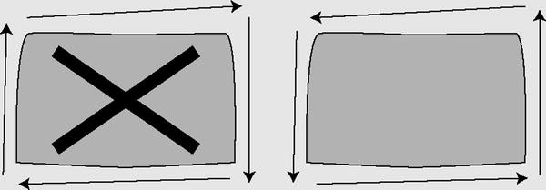
The next step is to tell SQL Server where the inside of the Polygon lies. SQL Server’s geography instance makes you define your coordinates in counterclockwise order, so the inside of the Polygon is everything that falls on the left-hand side of the lines connecting the coordinates. In the following illustration, the image on the left side is an invalid orientation because the coordinates are defined in a clockwise order. The image on the right side is a valid orientation because its coordinates are defined in a counterclockwise order. If you follow the direction of the arrows on the image, you’ll notice that the area on the left-hand side of the arrows is the area “inside” the Polygon. This eliminates any ambiguity from your Polygon definitions.
Keep these restrictions in mind if you decide to use the geography data type in addition to, or instead of, the geometry data type.
Polygon and MultiPolygon are two of the more interesting and complex spatial objects you can create. We like to use the state of Utah as a real-world example of a Polygon object for a couple of reasons. First, the exterior bounding ring for the state is very simple, composed of relatively straight lines. Second, the Great Salt Lake within the state can be used as a highly visible example of an interior bounding ring. Figure 10-20 shows the state of Utah.
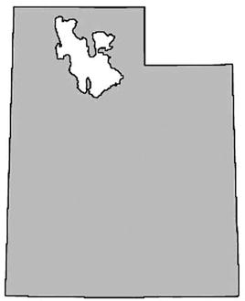
Figure 10-20. The state of Utah with the Great
The state of Michigan provides an excellent example of a MultiPolygon object. Michigan is composed of two distinct peninsulas, known as the Upper Peninsula and Lower Peninsula, respectively. The two peninsulas are separated by the Straits of Mackinac, which join Lake Michigan to Lake Huron. Figure 10-21 shows the Michigan MultiPolygon.

Figure 10-21. Michigan as a MultiPolygon Salt Lake as an Interior Bounding Ring
Michigan and the Great lakes
Michigan’s two peninsulas are separated by the Straits of Mackinac, which is a five-mile-wide channel that joins two of the Great Lakes, Lake Michigan and Lake Huron. Although these two bodies of water are historically referred to as separate lakes, hydrologists consider them to be one contiguous body of water. Hydrology experts sometimes refer to the lakes as a single entity, Lake Michigan-Huron. On the other hand, it makes sense to consider the two lakes as separate from a political point of view, since Lake Michigan is wholly within the borders of the United States, while the border between the United States and Canada divides Lake Huron. For the purposes of this section, the most important fact is that the lakes separate Michigan into two peninsulas, making it a good example of a MultiPolygon.
Through the use of the spatial instance types, you can create spatial objects that cover the entire range from very simple to extremely complex. Once you’ve created spatial objects, you can use the geometry and geography data type methods on them or create spatial indexes on spatial data type columns to increase calculation efficiency. Listing 10-28 uses the geography data type instance created in Listing 10-22 and the STIntersects() method to report whether the town of Laramie and the Statue of Liberty are located within the borders of Wyoming. The results are shown in Figure 10-22.
Listing 10-28. Are the Statue of Liberty and Laramie in Wyoming?
DECLARE @Wyoming geography,
    @StatueOfLiberty geography,
    @Laramie geography;

SET @Wyoming = geography::GeomFromGml ('<Polygon
    xmlns="http://www.opengis.net/gml">
    <exterior>
        <LinearRing>
        <posList>
        41.698246  -104.053108  41.999851       -104.053009
        43.003094  -104.05571  43.503738        -104.057426
        44.145844  -104.059242  44.574368       -104.058975
        45.001091  -105.04126  44.997227        -106.020576
        44.999813  -107.893715  44.997643       -108.624573
        45.002853  -109.994789  44.992348       -110.428894
        44.664562  -111.050842  43.982632       -111.049629
        43.284813  -111.04673  42.503323        -111.046028
        41.578648  -111.050323  40.996635       -111.050285
        40.997646  -110.001457  41.00341        -107.918037
        40.998489  -106.864838  41.000111       -106.202896
        40.994305  -104.933968  41.388107       -104.053505
        41.698246  -104.053108
        </posList>
        </LinearRing>
    </exterior>
</Polygon>', 4269);

SET @StatueOfLiberty = geography::GeomFromGml('<Point
    xmlns="http://www.opengis.net/gml">
    <pos>
        40.689124 -74.044483
    </pos>
    </Point>', 4269);

SET @Laramie = geography::GeomFromGml('<Point
    xmlns="http://www.opengis.net/gml">
    <pos>
        41.312928 -105.587253
    </pos>
    </Point>', 4269);

SELECT 'Is the Statue of Liberty in Wyoming?',
    CASE @Wyoming.STIntersects(@StatueOfLiberty)
        WHEN 0 THEN 'No'
        ELSE 'Yes'
    END AS Answer
UNION
SELECT 'Is Laramie in Wyoming?',
    CASE @Wyoming.STIntersects(@Laramie)
        WHEN 0 THEN 'No'
        ELSE 'Yes'
    END;

Figure 10-22. The Results of the STIntersection() Method Example
SQL Server also allows you to create spatial indexes that optimize spatial data calculations. Spatial indexes are created by decomposing your spatial data into a b-tree-based grid hierarchy four levels deep. Each level represents a further subdivision of the cells above it in the hierarchy. Figure 10-23 shows a simple example of a decomposed spatial grid hierarchy.

Figure 10-23. Decomposing Space for Spatial Indexing
The CREATE SPATIAL INDEX statement allows you to create spatial indexes on spatial data type columns. Listing 10-29 is an example of a CREATE SPATIAL INDEX statement.
Listing 10-29. Creating a Spatial Index
CREATE SPATIAL INDEX SIX_Location ON MyTable (SpatialColumn);
Spatial indexing is one of the biggest benefits of storing spatial data inside the database. As one astute developer pointed out, “Without spatial indexing, you may as well store your spatial data in flat files.”
![]() Note Pro Spatial with SQL Server 2012, by Alastair Aitchison (Apress, 2012), is a fully dedicated book about SQL Server Spatial, a feature much more complex that what we present here.
Note Pro Spatial with SQL Server 2012, by Alastair Aitchison (Apress, 2012), is a fully dedicated book about SQL Server Spatial, a feature much more complex that what we present here.
FILESTREAM Support
SQL Server is optimized for dealing with highly structured relational data, but SQL developers have long had to deal with heterogeneous unstructured data. The varbinary(max) LOB (Large Object) data type provides a useful method of storing arbitrary binary data directly in database tables; however, it still has some limitations, including the following:
- There is a hard 2.1 GB limit on the size of binary data that can be stored in a varbinary(max) column, which can be an issue if the documents you need to store are larger.
- Storing and managing large varbinary(max) data in SQL Server can have a negative impact on performance, owing largely to the fact that the SQL Server engine must maintain proper locking and isolation levels to ensure data integrity in the database.
Many developers and administrators have come up with clever solutions to work around this problem. Most of these solutions are focused on storing LOB data as files in the file system and storing file paths pointing to those files in the database. This introduces additional complexities to the system since you must maintain the links between database entries and physical files in the file system. You also must manage LOB data stored in the file system using external tools, outside of the scope of database transactions. Finally, this type of solution can double the amount of work required to properly secure your data, since you must manage security in the database and separately in the file system.
SQL Server provides a third option: integrated FILESTREAM support. SQL Server can store FILESTREAM-enabled varbinary(max) data as files in the file system. SQL Server can manage the contents of the FILESTREAM containers on the file system for you and control access to the files, while the NT File System (NTFS) provides efficient file streaming and file system transaction support. This combination of SQL Server and NTFS functionality provides several advantages when dealing with LOB data, including increased efficiency, manageability, and concurrency. Microsoft provides some general guidelines for use of FILESTREAM over regular LOB data types, including the following:
- When the average size of your LOBs is greater than 1 MB
- When you have to store any LOBs that are larger than 2.1 GB
- When fast-read access is a priority
- When you want to access LOB data from middle-tier code
![]() Tip For smaller and limited LOB data, storing the data directly in the database might make more sense than using FILESTREAM.
Tip For smaller and limited LOB data, storing the data directly in the database might make more sense than using FILESTREAM.
Enabling FILESTREAM Support
The first step to using FILESTREAM functionality in SQL Server is enabling it. You can enable FILESTREAM support through the SQL Server Configuration Manager. You can set FILESTREAM access in the SQL Server service Properties FILESTREAM page. Once you’ve enabled FILESTREAM support, you can set the level of access for the SQL Server instance with sp_configure and then restart the SQL Server service. Listing 10-30 enables FILESTREAM support on the SQL Server instance for the maximum allowable access.
Listing 10-30. Enabling FILESTREAM Support on the Server
EXEC sp_configure 'filestream access level', 2;
RECONFIGURE;
The configuration value defines the access level for FILESTREAM support. The levels supported are listed in Table 10-4.
Table 10-4. FILESTREAM Access Levels
|
Configuration Value |
Description |
|---|---|
|
0 |
Disabled (default) |
|
1 |
Access via T-SQL only |
|
2 |
Access via T-SQL and file system |
You can use the query in Listing 10-31 to see the FILESTREAM configuration information at any time. Sample results from our local server are shown in Figure 10-24.
Listing 10-31. Viewing FILESTREAM Configuration Information
SELECT
    SERVERPROPERTY('ServerName') AS ServerName,
    SERVERPROPERTY('FilestreamSharename') AS ShareName,
    CASE SERVERPROPERTY('FilestreamEffectiveLevel')
        WHEN 0 THEN 'Disabled'
        WHEN 1 THEN 'T-SQL Access Only'
        WHEN 2 THEN 'Local T-SOL/File System Access Only'
        WHEN 3 THEN 'Local T-SOL/File System and Remote File System Access'
    END AS Effective_Level,
    CASE SERVERPROPERTY('FilestreamConfiguredLevel')
        WHEN 0 THEN 'Disabled'
        WHEN 1 THEN 'T-SQL Access Only'
        WHEN 2 THEN 'Local T-SOL/File System Access Only'
        WHEN 3 THEN 'Local T-SOL/File System and Remote File System Access'
    END AS Configured_Level;
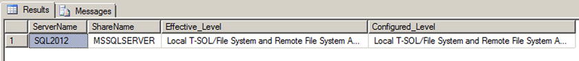
Figure 10-24. Viewing FILESTREAM Configuration Information
Creating FILESTREAM Filegroups
Once you’ve enabled FILESTREAM support on your SQL Server instance, you have to create an SQL Server filegroup with the CONTAINS FILESTREAM option. This filegroup is where SQL Server will store FILESTREAM LOB files. As AdventureWorks 2014 is shipped without a FILESTREAM filegroup, we need to add it manually. Listing 10-32 shows the final generated CREATE DATABASE statement as if we had created the database from scratch. The FILEGROUP clause of the statement that creates the FILESTREAM filegroup is shown in bold.
Listing 10-32. CREATE DATABASE for AdventureWorks Database
CREATE DATABASE [AdventureWorks]
 CONTAINMENT = NONE
 ON PRIMARY
( NAME = N'AdventureWorks2014_Data', FILENAME = N'C:sqldataMSSQL12.MSSQLSERVERMSSQLDATAAdventureWorks2014_Data.mdf', SIZE = 226304KB, MAXSIZE = UNLIMITED, FILEGROWTH = 16384KB ),
 FILEGROUP [FILESTREAM1] CONTAINS FILESTREAM  DEFAULT
( NAME = N'AdventureWordsFS', FILENAME = N'C:sqldataMSSQL12.MSSQLSERVERMSSQLDATAAdventureWordsFS', MAXSIZE = UNLIMITED)
 LOG ON
( NAME = N'AdventureWorks2014_Log', FILENAME = N'C:sqldataMSSQL12.MSSQLSERVERMSSQLDATAAdventureWorks2014_log.ldf', SIZE = 5696KB, MAXSIZE = UNLIMITED, FILEGROWTH = 10%);
To create this FILESTREAM filegroup on an already existing database, we used the ALTER DATABASE statement as shown in Listing 10-33.
Listing 10-33. Adding a FILESTREAM Filegroup to an Existing Database
ALTER DATABASE AdventureWorks
ADD FILEGROUP FILESTREAM1 CONTAINS FILESTREAM;
GO
ALTER DATABASE AdventureWorks
ADD FILE
(
NAME = N' AdventureWordsFS',
FILENAME = N' C:sqldataMSSQL12.MSSQLSERVERMSSQLDATAAdventureWordsFS' )
TO FILEGROUP FILESTREAM1;
You can see that the file created is in fact not a file, but a directory where the files will be stored by SQL Server.
Once you’ve enabled FILESTREAM on the server instance and created a FILESTREAM filegroup, you’re ready to create FILESTREAM-enabled tables. FILESTREAM storage is accessed by creating a varbinary(max) column in a table with the FILESTREAM attribute. The FILESTREAM-enabled table must also have a uniqueidentifier column with a ROWGUIDCOL attribute and a unique constraint on it. The Production.Document table in the AdventureWorks sample database is ready for FILESTREAM. In fact, its Document column was declared as a varbinary(max) with the FILESTREAM attribute in AdventureWorks 2008, but this dependency was removed in AdventureWorks 2012. Now, the Document column is still a varbinary(max), and the rowguid column is declared as a uniqueidentifier with the ROWGUIDCOL attribute. To convert it to a FILESTREAM-enabled table, we create a new table named Production.DocumentFS and import the lines from Production.Document into that new table. Let’s see how it works in Listing 10-34. The Document and rowguid columns are shown in bold.
Listing 10-34. Production.Document FILESTREAM-Enabled Table
CREATE TABLE Production.DocumentFS (
    DocumentNode    hierarchyid NOT NULL PRIMARY KEY,
    DocumentLevel   AS (DocumentNode.GetLevel()),
    Title           nvarchar(50) NOT NULL,
    Owner           int NOT NULL,
    FolderFlag      bit NOT NULL,
    FileName        nvarchar(400) NOT NULL,
    FileExtension   nvarchar(8) NOT NULL,
    Revision        nchar(5) NOT NULL,
    ChangeNumber    int NOT NULL,
    Status          tinyint NOT NULL,
    DocumentSummary nvarchar(max) NULL,
    Document        varbinary(max) FILESTREAM NULL,
    rowguid         uniqueidentifier ROWGUIDCOL NOT NULL UNIQUE,
    ModifiedDate    datetime NOT NULL
);
GO

INSERT INTO Production.DocumentFS
    (DocumentNode, Title, Owner, FolderFlag, FileName, FileExtension, Revision, ChangeNumber, Status, DocumentSummary, Document, rowguid, ModifiedDate)
SELECT
    DocumentNode, Title, Owner, FolderFlag, FileName, FileExtension, Revision, ChangeNumber, Status, DocumentSummary, Document, rowguid, ModifiedDate
FROM Production.Document;
When the table is created, we insert the content of Production.Document into it. Now, we can open Windows Explorer and go to the location of the FILESTREAM directory. The content of the directory is shown in Figure 10-25. The file names appear as a jumble of grouped digits that don’t offer up much information about the LOB files’ contents, because SQL Server manages the file names internally.

Figure 10-25. LOB Files Stored in the FILESTREAM Filegroup
![]() Caution SQL Server also creates a file named filestream.hdr. This file is used by SQL Server to manage FILESTREAM data. Do not open or modify this file.
Caution SQL Server also creates a file named filestream.hdr. This file is used by SQL Server to manage FILESTREAM data. Do not open or modify this file.
Accessing FILESTREAM Data
You can access and manipulate your FILESTREAM-enabled varbinary(max) columns using standard SQL Server SELECT queries and DML statements like INSERT and DELETE. Listing 10-35 demonstrates querying the varbinary(max) column of the Production.DocumentFS table. The results are shown in Figure 10-26.
Listing 10-35. Querying a FILESTREAM-Enabled Table
SELECT
    d.Title,
    d.Document.PathName() AS LOB_Path,
    d.Document AS LOB_Data
FROM Production.DocumentFS d
WHERE d.Document IS NOT NULL;

Figure 10-26. Results of Querying the FILESTREAM-enabled Table
A property called PathName() is exposed on FILESTREAM-enabled varbinary(max) columns to retrieve the full path to the file containing the LOB data. The query in Listing 10-35 uses PathName() to retrieve the LOB path along with the LOB data. As you can see from this example, SQL Server abstracts away the NTFS interaction to a large degree, allowing you to query and manipulate FILESTREAM data as if it were relational data stored directly in the database.
![]() Tip In most cases, it’s not a good idea to retrieve all LOB data from a FILESTREAM-enabled table in a single query as in this example. For large tables with large LOBs, this can cause severe performance problems and make client applications unresponsive. In this case, however, the LOB data being queried is actually very small in size, and there are few rows in the table.
Tip In most cases, it’s not a good idea to retrieve all LOB data from a FILESTREAM-enabled table in a single query as in this example. For large tables with large LOBs, this can cause severe performance problems and make client applications unresponsive. In this case, however, the LOB data being queried is actually very small in size, and there are few rows in the table.
SQL Server 2008, 2012 and 2014 provide support for the OpenSqlFilestream API for accessing and manipulating FILESTREAM data in client applications. A full description of the OpenSqlFilestream API is beyond the scope of this book, but Accelerated SQL Server 2008, by Rob Walters et al. (Apress, 2008), provides a description of the OpenSqlFilestream API with source code for a detailed client application.
SQL Server 2012 improved greatly the FILESTREAM type by introducing filetables. As we have seen, to use FILESTREAM we need to manage the content only through SQL Server, by T-SQL or with the OpenSqlFilestream API. It is unfortunate, because we have access to a directory on our file system, which cannot be managed simply and publishes cryptic file names. In short, we have a great functionality that could be more flexible and user-friendly. Filetable brings that to the table. It makes the Windows filesystem namespace compatible with SQL Server tables. With it, you can create a table in SQL Server that merely reflects the content of a directory and its subdirectories, and you can manage its content at the file system level, out of SQL Server, with regular tools like the Windows Explorer, or by file I/O APIs in your client application. All changes made to the file system will be immediately reflected in the filetable. In fact, the file system as we see it in the share does not exist per se; it is a kind of mirage created by SQL Server. Files or directories will be internally handled by SQL Server and filestream objects, and if you try to access the real directory with Windows Explorer, it will be as jumbled as any other FILESTREAM directory.
To be able to use filetables, you first need to have activated the filestream support at the instance level as we have seen in the previous section. The filestream_access_level option needs to be set to 2 to accept file I/O streaming access. In addition, the FILESTREAM property of the database must be set to accept non-transacted access. We will see how to do that in our example. We have downloaded a zip package from the http://openclipart.org/ web site, containing the entire collection of free cliparts. It represents almost 27,000 image files at this time. We will add them in a filetable. First, in Listing 10-36, we create a dedicated database with a FILESTREAM filegroup that will store our filetable. The FILESTREAM filegroup creation is shown in bold.
Listing 10-36. Creating a Database with a FILESTREAM Filegroup
CREATE DATABASE cliparts
CONTAINMENT = NONE
ON PRIMARY
( NAME = N'cliparts', FILENAME = N'C:sqldataMSSQL12.MSSQLSERVERMSSQLDATAcliparts.mdf', SIZE = 5120KB, FILEGROWTH = 1024KB ),
FILEGROUP [filestreamFG1] CONTAINS FILESTREAM
( NAME = N'filestream1', FILENAME = N'C:sqldataMSSQL12.MSSQLSERVERMSSQLDATAfilestream1' )
LOG ON
( NAME = N'cliparts_log', FILENAME = N'C:sqldataMSSQL12.MSSQLSERVERMSSQLDATAcliparts_log.ldf', SIZE = 1024KB , FILEGROWTH = 10%);
GO

ALTER DATABASE [cliparts] SET FILESTREAM( NON_TRANSACTED_ACCESS = FULL, DIRECTORY_NAME = N'cliparts' );
![]() Note As filetables are stored in a FILESTREAM filegroup, filetables are included in database backups, unless you perform filegroup backups and you exclude the FILESTREAM filegroup.
Note As filetables are stored in a FILESTREAM filegroup, filetables are included in database backups, unless you perform filegroup backups and you exclude the FILESTREAM filegroup.
In the last line of Listing 10-36, we set the filestream option to NON_TRANSACTED_ACCESS = FULL, which will ensure that files will be writable from the share outside of SQL Server. We also specify the directory name 'cliparts'. It will be shown as a sub-directory in the FILESTREAM share.
The path where a filetable will be found on the share depends on the directory set at the database level, plus a sub-directory set when the table is created. In Listing 10-37, we create the filetable and a directory by inserting a line in the filetable.
Listing 10-37. Creating the Filetable
USE [cliparts];
GO

CREATE TABLE dbo.OpenClipartsLibrary AS FILETABLE
WITH
    (
        FILETABLE_DIRECTORY = 'OpenClipartsLibrary'
    );
GO

INSERT INTO dbo.OpenClipartsLibrary (name,is_directory)
VALUES ('import_20120501',1);
To create a filetable, we simple create a table AS FILETABLE. We specify with the option FILETABLE_DIRECTORY = 'OpenClipartsLibrary' in which directory in the share the content of the table will be found.
![]() Note The directory of a filetable can be changed later with an ALTER TABLE.
Note The directory of a filetable can be changed later with an ALTER TABLE.
As you can see, the table structure is not part of the CREATE TABLE statement. A filetable schema is fixed. We describe the filetable columns in Table 10-5.
Table 10-5. Filetable Structure
|
Column |
Type |
Description |
|---|---|---|
|
stream_id |
uniqueindetifier |
The unique id of the line, being a file (a FILESTREAM document) or a directory. There is a UNIQUE constraint on it. |
|
file_stream |
varbinary(max) |
The FILESTREAM column containing the file. NULL if it is a directory. |
|
name |
nvarchar(255) |
Contains the name of the file or directory. |
|
path_locator |
hierarchyid |
The position of the file or directory in the directory’s hierarchy. The primary key of the table. |
|
parent_path_locator |
hierarchyid |
The path_locator of the parent (ie., the directory containing the file or directory). A calculated column. |
|
file_type |
nvarchar(255) |
The type (extension) of the file. A calculated column. NULL if it is a directory. |
|
cached_file_size |
bigint |
The size of the file in bytes. A calculated column. NULL if it is a directory. |
|
creation_time |
datetimeoffset(7) |
The date and time of creation. It is set by default at the current date and time when the object is created. |
|
last_write_time |
datetimeoffset(7) |
The date and time of the last modification of the file or directory. Can be set manually like creation_time. |
|
last_access_time |
datetimeoffset(7) |
The date and time when the file was last accessed. Can be set manually like creation_time. |
|
is_directory |
bit |
1 if it is a directory. Calculated. |
|
is_offline |
bit |
1 if the extended NTFS attribute Offline is set on the file. That would mean that the file is not physically in the directory but stored remotely. |
|
is_hidden |
bit |
1 if the file has the hidden attribute. |
|
is_readonly |
bit |
1 if the file has the read-only attribute. |
|
is_archive |
bit |
1 if the file has the archive bit set. |
|
is_system |
bit |
1 if the file has the system attribute. |
|
is_temporary |
bit |
1 if the file has the temporary attribute. |
To retrieve the filetables in our database, we can query the sys.filetables catalog view. We also can find them in SSMS Object Explorer, in the Tables | FileTables node, as shown in Figure 10-27.
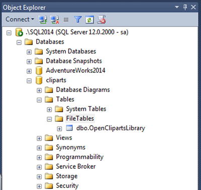
Figure 10-27. Filetables in SSMS
You can see the share itself in Windows Explorer by going to Network, choosing your server name and entering the share name you set in the SQL Server Configuration Manager. You can also right-click on the filetable in the SSMS Object Explorer—as we see in Figure 10-27—and click on “Explore FileTable Directory,” which will open a Windows Explorer window directly on the filetable directory. You need to access it through the network share, and not directly through the local directory, because the local directory will only show you FILESTREAM GUID names, while the network share, managed by SQL Server, will show you a virtual directory hierarchy that looks like a regular hierarchy of directores and files. This is logical anyway, as clients are not supposed to access directly local server directories. For our example, we did that and copied the full unzipped cliparts directory and subdirectories. When the copy was finished, a COUNT(*) from dbo.OpenClipartsLibrary returned 27,890 lines.
To manage files and directories, you can do it by issuing T-SQL statements against the filetable, directly in the share with Windows tools, or programmatically with Windows I/O APIs. As an example of how to do it also by T-SQL, Listing 10-38 creates a new directory under the OpenClipartsLibrary root directory.
Listing 10-38. Inserting a Directory in the Filetable
INSERT INTO dbo.OpenClipartsLibrary (name, is_directory)
VALUES ('directory01',1);
Setting the is_directory column to 1 is all you have to do to create a directory. You can also modifiy the file or directory properties by Windows I/O APIs or by T-SQL queries against the table. In Listing 10-39, we insert a subdirectory or the newly created directory01 and set a creation date as different from the current date and time.
Listing 10-39. Inserting a Subdirectory
INSERT INTO dbo.OpenClipartsLibrary
     (name, is_directory, creation_time, path_locator)
SELECT
    'directory02',1, dateadd(year, -1, sysdatetime()), path_locator.GetDescendant(NULL, NULL)
FROM dbo.OpenClipartsLibrary
WHERE name = 'directory01'
AND is_directory = 1
AND parent_path_locator IS NULL;
The code in Listing 10-39 creates a directory named directory02 as a subdirectory of directory01 by setting the path_locator of the created directory with the GetDescendant() hierarchyId method of the directory01 path_locator column. GetDescendant(NULL, NULL) returns the least descendant node of the current hierarchyId value. To be sure that directory01 is the one we created at the root level, we check that its parent_path_locator is NULL. We also set manually the creation_date to be one year ago.
In Figure 10-28, we verify with Windows Explorer that the directory was effectively created. Once again, you need to do it through the network share.

Figure 10-28. The Newly Created Directory02 Directory
![]() Note You cannot change a file to be a directory or vice versa. A check constraint on the filetable enforces that is_directory cannot be set to 1 when the file_stream column is not NULL.
Note You cannot change a file to be a directory or vice versa. A check constraint on the filetable enforces that is_directory cannot be set to 1 when the file_stream column is not NULL.
Whenever you add, move or delete a file on the share, or by T-SQL statements against the filetable, it will be immediately reflected at both places. SQL Server intercepts all I/O operations on the share and converts them into DML actions on the filetable. File system rules like name limitations are enforced by constraints on the filetable, and trying to create invalid files or folders (with names containing / ? < > : * | ”) in the filetable will result in a constraint violation.
There is however an important difference between managing the filetable content by T-SQL or at the Windows level. The DML statements against a filetable can be part of a transaction and rolled back, while creating, modifying, moving, or deleting files and folders by the means of the Windows I/O APIs cannot be part of a transaction. That’s the reason why we enabled non_transacted_access support in our database. If you want to enable transactional modification of a file in a filetable outside of T-SQL context, you can use the OpenSqlFileStream API in your client code, which we discussed previously.
You can use dedicated functions, FILESTREAM related functions, and hierarchyid functions to manipulate files and folders in a filetable.
The FileTableRootPath() function returns the database share directory if called without argument, or the filetable share directory if called with the name of a filetable provided in a nvarchar argument, as shown in Listing 10-40. The results are shown in Figure 10-29.
Listing 10-40. Using FileTableRootPath()
USE cliparts;

SELECT FileTableRootPath();
SELECT FileTableRootPath('dbo.OpenClipartsLibrary'),
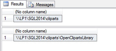
Figure 10-29. The Results of FileTableRootPath()
The function takes a second optional parameter, @option, which is useful to return the full path in NETBIOS format or with the full domain name (FDN) of the server. The @option possible values are detailed in Table 10-6.
Table 10-6. FileTableRootPath @options
|
@option value |
Description |
|---|---|
|
0 |
Returns the path in NETBIOS format; this is the default value. A NETBIOS computer name has a maximum of 16 characters in uppercase. |
|
1 |
Returns the path without conversion. |
|
2 |
Returns the path with the full domain name (FDN) of the machine. |
To get the path of a specific file or folder in the filetable, the GetFileNamespacePath() function comes in handy. It is called as a method of the file_stream column, and takes two optional parameters, the first, @is_full_path, allows the path returned to be relative (0) or absolute (1). Calling GetFileNamespacePath(1) will produce full paths and saves you from concatenating the result of FileTableRootPath() with the relative path. The second option, @option, has the same values as the @option parameter of the FileTableRootPath() function. We demonstrate the usage of GetFileNamespacePath() in Listing 10-41.
Listing 10-41. Using GetFileNamespacePath(),
SELECT file_stream.GetFileNamespacePath(1) as path
FROM dbo.OpenClipartsLibrary
WHERE is_directory = 1
ORDER BY path_locator.GetLevel(), path;
The statement in Listing 10-41 returns all the directories of absolute paths ordered by their level in the directories’ hierarchy and their name. The GetLevel() hierarchyid function applied to the path_locator column allows you to return the current level of the item in the file system relative to the filetable root.
As we can see, hierarchyid functions are interesting ways to move through the hierarchy. An example is given in Listing 10-42 that returns a directory and the name of its parent directory. A partial result is shown in Figure 10-30.
Listing 10-42. Using hierarchyid Functions
SELECT l1.name, l1.path_locator.GetLevel(), l2.name as parent_directory
FROM dbo.OpenClipartsLibrary l1
JOIN dbo.OpenClipartsLibrary l2 ON l1.path_locator.GetAncestor(1) = l2.path_locator
WHERE l1.is_directory = 1;

Figure 10-30. The Results of Using hierarchyid Functions
By using the GetAncestor() hierarchyid function on the path_locator in the JOIN clause, we retrieve the parent path_locator and display its name. An easier way to do that is to use directly the parent_path_locator computed column that maintains a foreign key relationship with the path_locator column in the same table. The query in Listing 10-43 returns exactly the same result as the query in Listing 10-42.
Listing 10-43. Using Parent_path_locator Column
SELECT l1.name, l1.path_locator.GetLevel(), l2.name as parent_directory
FROM dbo.OpenClipartsLibrary l1
JOIN dbo.OpenClipartsLibrary l2 ON l1.parent_path_locator = l2.path_locator
WHERE l1.is_directory = 1;
Thanks to the recursive relationship between parent_path_locator and path_locator, we can travel down the directory’s path with a recursive Common Table Expression (CTE), as follows in Listing 10-44.
Listing 10-44. Using a CTE to Travel Down the Directories’ Hierarchy
;WITH mycte AS (
    SELECT name, path_locator.GetLevel() as Level, path_locator
    FROM dbo.OpenClipartsLibrary
    WHERE name = 'Yason'
    AND is_directory = 1

    UNION ALL

    SELECT l1.name, l1.path_locator.GetLevel() as Level, l1.path_locator
    FROM dbo.OpenClipartsLibrary l1
    JOIN mycte l2 ON l1.parent_path_locator = l2.path_locator
    WHERE l1.is_directory = 1
)
SELECT name, Level
FROM mycte
ORDER BY level, name;
Of course, as the path_locator column is a hierarchyid, we might as well express it as in Listing 10-45.
Listing 10-45. Using hierarchyid Functions to Travel Down the Directory’s Hierarchy
SELECT l1.name, l1.path_locator.GetLevel() as Level
FROM dbo.OpenClipartsLibrary l1
JOIN dbo.OpenClipartsLibrary l2 ON l1.path_locator.IsDescendantOf(l2.path_locator) = 1 OR
l1.path_locator = l2.path_locator
WHERE l1.is_directory = 1
AND l2.is_directory = 1
AND l2.name = 'Yason'
ORDER BY level, name;
In Listing 10-45, we use the IsDescendantOf()function to retrieve all descendent directories of the directory named Yason. We have copied a few directories in Yason, and the queries in Listings 10-44 and 10-45 return exactly the same result shown in Figure 10-31.
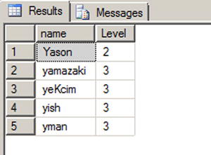
Figure 10-31. The Results of the Queries in Listings 10-44 and 10-45
Finally, the GetPathLocator() function returns a path_locator value for a file system full path. The example in Listing 10-46 retrieves the path_locator of the Yason directory, and uses it to find the matching line in the OpenClipartsLibrary table. The result is shown in Figure 10-32.
Listing 10-46. Using the GetPathLocator() function.
DECLARE @path_locator hierarchyid

SET @path_locator = GetPathLocator('\Sql2012mssqlserverclipartsOpenClipartsLibrary
import_20120501Yason'),

SELECT *
FROM dbo.OpenClipartsLibrary
WHERE path_locator = @path_locator;

Figure 10-32. The Line Found Using the GetPathLocator() Function
Filetables can have triggers like any other tables. Because making changes in the filetable share at the Windows level results in SQL Server calls behind the scene, a trigger will also receive these events.
![]() Note But replication and related features (including transactional replication, merge replication, change data capture, and change tracking) are not supported with FileTables. You can see a FileTable Compatibility list with SQL Server features at this address: http://msdn.microsoft.com/en-us/library/gg492086.aspx.
Note But replication and related features (including transactional replication, merge replication, change data capture, and change tracking) are not supported with FileTables. You can see a FileTable Compatibility list with SQL Server features at this address: http://msdn.microsoft.com/en-us/library/gg492086.aspx.
We will demonstrate that with the audit table and the trigger created in Listing 10-47.
Listing 10-47. Creating an Audit Table and a Trigger on the OpenClipartsLibrary Table
CREATE TABLE dbo.cliparts_log (
    path nvarchar(4000) not null,
    deletion_date datetime2(0),
    deletion_user sysname,
    is_directory bit
)
GO

CREATE TRIGGER OpenClipartsLibrary_logTrigger
ON [dbo].[OpenClipartsLibrary]
AFTER DELETE
AS BEGIN
    IF @@ROWCOUNT = 0 RETURN;
    SET NOCOUNT ON;

    INSERT INTO dbo.cliparts_log (path, deletion_date, deletion_user, is_directory)
    SELECT name, SYSDATETIME(), SUSER_SNAME(),is_directory
    FROM deleted
END;
First, we create an audit table named cliparts_log. We want to keep track of file and directory deletions. We want to keep the date and time of deletion and name of the account that deleted the item. To record deletion into the table, we create a trigger named OpenClipartsLibrary_logTrigger that will fire for every DELETE statement against the OpenClipartsLibrary table.
To test it, we go to the filetable share with Windows Explorer and delete the \Sql2014mssqlserverclipartsOpenClipartsLibraryimport_20140501acspike directory. It contains two files. What gets written in the table is shown in Figure 10-33.
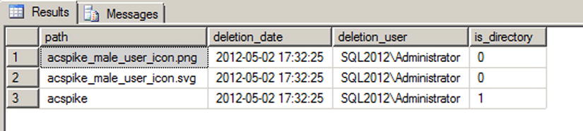
Figure 10-33. The Content of the Cliparts_log Table after the Directory’s Deletion
Summary
In this chapter, we first discussed some details to know about basic data types. Mastering how basic data types work allows you to understand the impact they have on the storage, and therefore on the performance, of your database. For instance, the nvarchar data type stores UNICODE values and consumes twice the space of the same varchar content. If used lightly, it can blow up the size of your database file. The varchar(max) and varbinary(max) types replace the legacy text and image data types. They allow an easy and more performant handling on Large Objects (LOB) inside the database. We then spent some time on the date and time data types. They have been improved in SQL Server 2008 with new types that are more precise and compact.
We also covered more advanced data types, like uniqueidentifier, which stored a 16-byte globally unique identifier, and hierarchyid, a .NET-based data type that can be used in a hierarchical table to represent a tree structure, as well as the spatial geometry and geography data types.
Finally, we explored the FILESTREAM type. With FILESTREAM, you can keep binary documents inside a database more efficiently. Through SQL Server, the document will be stored in the NTFS file system and can be retrieved directly with I/O APIs. Transactional coherence is maintained on the files as if they were inside the database file. The new filetable feature improves upon FILESTREAM by offering special database tables storing FILESTREAM documents and folder definitions that can be accessed simply on the filesystem with a network share managed by SQL Server.
EXERCISES
- [True/False] Storing character strings with European language accents (é,à, ö, for instance) requires you to use a UNICODE encoding.
- [Choose all that apply] Which of the following LOB data types are deprecated?
- image
- varchar(max)
- text
- ntext
- All of the above
- [True/False] The new date data type stores time offset information.
- What model does the hierarchyid data type use to represent hierarchical data in the database?
- [Choose one] Which of the following is true of Polygon spatial objects when created in geography data type instances?
f. They must have a clockwise orientation.
g. They must have a counterclockwise orientation.
h. Orientation does not matter.
i. They cannot cross up to two hemispheres.
- [Choose one] Which of the following functions adjusts a given datetimeoffset value to another specified time offset?
j. TODATETIMEOFFSET
k. SWITCHOFFSET
l. CHANGEOFFSET
m. CALCULATE OFFSET
- [True/False] The FILESTREAM functionality in SQL Server 2014 uses NTFS to provide streaming LOB data support.
- What is the name of the filetable column that allows you to retrieve the path of the file or directory on the filetable network share?