![]()
Introduction to Simulation
In many cases, to understand the dynamics of a real world system or a function of a physical system, we need to model it and imitate the step by step operation of the system using a computational tool. This step by step imitation of a real world process is known as simulation. The systems can include any physical phenomena such as Brownian motion or the path of a projectile; or man-made devices such as robots or motors. Computational tools developed for simulating a system can be based on hardware or software. In this chapter, we will learn how to simulate in a software-based computation tool, in particular in MATLAB.
One Step Simulations
Although real world processes are infinite time processes, sometimes they can be regarded as one time computations. For example, suppose a projectile is thrown into the sky with velocity ![]() from the ground.
from the ground.
If we want to know the motion of this projectile or the range covered by it, even though the process evolves with time, we can compute it in one step using motion equations:
Location path:

and this can be plotted easily using the following code (see Figure 5-1):
v=[10 20];
g=9.8;
%flight time
flighttime=2(v(2))/g;
%range
r=v(1)*flighttime;
%plot projectile path
t=[0:flighttime/100:flighttime];
plot(v(1)*t,v(2)*t-0.5*g*t.^2);
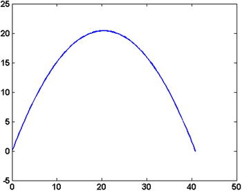
Figure 5-1. Simulated path of a projectile
However, when the motion is complex, e.g. affected by many forces or collisions, it is very hard to compute the equations of the path. In such cases we need to simulate the process at small time steps to see how each object moves in each instant. We will see how we can simulate projectile motion using iterative simulations in later sections of this chapter.
In this section, we will consider a simple example from optics which will illustrate the basic technique of one step simulation. Let us assume a point located at x = a, y = 0. A plane mirror is positioned in the YZ plane at y=0. To compute the reflection, we will take two rays originating from the point and find its reflected ray and finally compute the intersection to find the image (Figure 5-2 shows the results).
%Location of the point
a=10;x1=[a 0];
%take first line at theta =120, line in the format y=m1x+c1
t1=120;m1=tand(t1);
c1=0-m1*a;
%hitting point at mirror
A=[0 0*m1+c1];
%reflected light y=mr1x+cr1
mr1=tand(180-t1);cr1=A(2)-  mr1*A(1);
%second ray at t=150
t2=150;m2=tand(t2);
c2=0-m2*a;B=[0 0*m2+c2];
mr2=tand(180-t2);cr2=B(2)-  mr2*B(1);
%intersection of y=mr1x+cr1 and y=mr2x+cr2
xr=(cr2-cr1)/(mr1-mr2);
yr=xr*mr1+cr1;
disp([xr yr]);

Figure 5-2. Ray tracing diagram for a point object in front of a plane mirror
Iterative Methods
First, as a warm up exercise, we discuss some numerical methods which require iterations to be performed. Let us take a simple example of computing the zeros of the following equation:
![]()
There are many techniques available to solve equations of the form f (x)=0. One of them is the Newton-Raphson method, which is performed as follows:
- We begin with a first guess x0.
- A better solution of the equation x1, can be computed as

- Compute f (x1) and, if it is close enough to 0, terminate the algorithm and output x1.
- Now put x0 = x1 and compute x1 again by returning to step 2.
The algorithm is terminated when f (x1) is close enough to zero, let us say when | f (x1)|<∈f where ∈f is known as the function tolerance and can be arbitrarily defined according to the precision required. In this example, we set it to be equal to 0.001. There can be other termination conditions too, for example, we can terminate the algorithm when the value of x varies by a small difference in two consecutive iterations, in other words if |x1-x0|<∈x. Here ∈x is known as the x tolerance. The tolerance can also be defined in relative rather than absolute terms. For example, we can terminate the algorithm when

Let us first define the function and its derivative along with some parameters.
f=@(x) x.*sin(x)-0.2;
fprime=@(x) sin(x)+x.*cos(x);
x_0=0.1;
tolerance=0.001;
To implement the algorithm, we will first implement a single step, computing x1 from x0
x_1=x_0-f(x_0)/fprime(x_0);
Let us compute the error value of this step
err_step=abs(f(x_1));
Note that if we were using the x tolerance, the err_step would be
err_step=abs(x_1-x_0);
Now for the next step, we need to assign the value of x0 to x1 so that the previous line of code can be used again for the next step when computing the next x1.
x_0=x_1;
The whole step will look like
x_1=x_0-f(x_0)/fprime(x_0);
err_step=abs(f(x_1));
x_0=x_1;
Now this step can be repeated until the tolerance condition is met. The final value of x1 will be the solution. The whole code would look like the following
f=@(x) x.*sin(x)-0.2;
fprime=@(x) sin(x)+x.*cos(x);
x_0=0.1;
tolerance=0.001;
err_step=100;
while(err_step>tolerance)
        x_1=x_0-f(x_0)/fprime(x_0);
        err_step=abs(f(x_1));
        x_0=x_1;
end
final_sol=x_1;
When we run the above code, we get the answer as 0.4551.
Simulation of Real World Processes
In the previous section, we have seen how to implement an iterative method. Most real world processes are finite or infinite iterations of some steps. Let us first concentrate on discrete processes.
Discrete Processes
A discrete process x[n] is generally represented in the following two forms:
- Explicit expression of the value of the process at time n as x[n].
For example: x[n]= sin2πn.
- Definition of x[n] in terms of values at previous time steps, known as a time update equation.
For example:
 .
.
We will concentrate on the second definition as the first one is trivial. The following are the important steps used to simulate any real world process.
- Understand the process and make a mathematical model to compute the time step update equation.
- Model/generate or acquire the input signal.
- Implement one time step.
- Repeat the iterations for the desired time duration.
The following subsections discuss some examples of discrete random processes.
Random Walks
A random walk is a walk or series of steps where each step taken by the object is independent of all previous steps. It is also known as a drunken walk, where the person does not know where to go and each step taken by him is random. We will consider the discrete case in 2D space where four possible steps are allowed:
- [ 1 0] : unit step in the direction of the positive X axis
- [-1 0] : unit step in the direction of the negative X axis
- [ 0 1] : unit step in the direction of the positive Y axis
- [ 0 -1] : unit step in the direction of the negative Y axis
At each time step, the object chooses a number randomly out of {1,2,3,4} and depending on that number, it will take a step in the corresponding direction. A similar process is followed at each time step and this continues indefinitely. The random walk is the basis of many natural processes, such as Brownian motion.
The update equation is given as
![]()
Here r[n] is the location of the point at time step n
![]()
and w[n] is a random number with value between 1 to 4.
Since it is an iterative process, we will need to use a loop for its simulation. We will first simulate a single step, then we will put a loop around it. A single time step at time n consists of the following four sub-steps.
- Assign the current position .
- Generate a random number w[n] to select the direction of motion, which requires two bits [w1w2] of a random Bernoulli variable. These two values combined will select the direction as follows:
b=rand(1,2);
w=b>0.5;
if w==1
              rstep=[1 0];
elseif w(1)==1
        rstep=[0 1];
elseif w(2)==1
        rstep=[-1 0];
else
       rstep=[0 -1];
end
Remember if you put w==1 as a condition inside the if statement, it will be considered true only when all the elements in b satisfy the condition.
- Update the position with this new value:
rnew=r+rstep;
After we are done with one time step, we can put a loop around it to make it an iterative process and let it run for, let us say, 1000 time steps. We initialize r as the origin before the first time step.
r=[0 0];
for t= 0:0.1:100
                     b=rand(1,2);
                     w=b>0.5;
                     if w==1
                             rstep=[1 0];
                     elseif w(1)==1
                             rstep=[0 1];
                     elseif w(2)==1
                               rstep=[-1 0];
                     else
                               rstep=[0 -1];
                     end
      rnew=r+rstep;
      r=rnew;
end
Animation of the walk
Using the animation techniques learnt in previous chapters, we can also visualize the random walk by plotting each step as a line connecting the previous location to the new one.
plot([r(1) rnew(1)],[r(2) rnew(2)]);
Since we are adding each step to the previous trace, we need to use hold on at least once so that the previous steps are not deleted.
hold on;
plot([r(1) rnew(1)],[r(2) rnew(2)]);
drawnow
When we run this code, we will get Figure 5-3. We can increase the time limit by changing the for loop time vector.

Figure 5-3. Simulation of a random walk
Adding Drift
In the plot you can see that, as time passes, the object starts to return to the origin. It never stays at the origin, but it has the tendency to move around the origin and the expected distance from the origin at t=∞ is 0. This is because the selection of each direction is equally probable. For example, the probability that the [1 0] direction is chosen is given as
![]()
![]()

Now let us change the probabilities and observe its effect. We can change the direction selection step as follows:
    b=rand(1,2);
    w=b>[0.4 0.3];
Now we are comparing b1 with 0.4 and b2 with 0.3. So the probability of selecting the +X direction is given by
![]()
and so forth. The result is shown in Figure 5-4. We can clearly see a tendency of the walk to move in the +XY directions. This illustrates the motion of the object when a drifting force exists in the medium.

Figure 5-4. Simulation of a random walk with drift
Simulation of Continuous Time Processes
A continuous time process x(t) can again be represented mainly in two ways:
- Explicit form, for example

- Time update equations
Here the rate of change of the process describes its dynamics. For example, consider a process x(t) defined by

where w(t) is the input signal.
The first form is trivial, as before, so we concentrate on the second form. The first task when simulating such systems is to convert the system to a discrete time system via the following steps:
- Fix a sample time interval δ and sample the system with time step δ

where t0 is the start of the world, typically taken as 0.
- Next replace the derivate terms by the first principle definition of differentiation
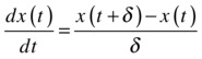
Thus, using the sample time definition, x(t+δ) can be written as
![]()
Let us work on the above mentioned example. The time update equation can be written as


![]()
which is in the same format as the discrete system discussed in the previous section and can be simulated in a similar way. We can actually save the whole process with respect to time instead of just keeping the current value. Recall that, in the previous example, at each step we updated r to rnew. At the end of the simulation, you don’t have access to the locations at previous times. In the following code, we will save all the values in a matrix x where the nth element of the matrix represents x[n]. We also assume that the input w(t) is zero. (See Figure 5-5.)
x(1)=[0];
delta=0.1;
for i= 1:100
      x(i+1)=x(i)+delta*(cos(delta*i)+2*exp(-delta*i)+0.4);
end
plot(1:101,x);

Figure 5-5. Simulation of a continuous time process
Let us now see how we can compute the motion of a projectile as discussed in the first section. At any time step, the update in velocity is given as
![]()
![]()
and the location is updated as
![]()
![]()
The simulation should terminate when the ball hits the ground, i.e. when xy is less than zero.
v=[10 20];g=9.8;x=[0 0];
delta=0.1;t=0;
while (x(2)>=0)
       v=v+[0 -g*delta];
       x=x+v*delta;
       plot(x(1),x(2),'ro','MarkerSize',6);
hold on;
axis([0 60 0 40])
drawnow;
t=t+delta;
end
flighttime=t;
range=x(1);
Example: Balls in a 2D Box
Let us consider a complex example. Suppose there are N balls in a 2D plane, given initial velocities and confined within some boundary (-L ≤ x, y≤ L). As the balls move in a plane, if they collide with other balls, they exchange their velocities and continue moving. If they hit the boundary, they reverse their component of velocity, which is in the direction of confinement. For example, if they hit x=L, their velocity will change as
![]()
![]()
We are interested in simulating this system for two minutes with a time interval of 0.1s, which corresponds to 1200 time step evaluations as

To simulate this, we follow the same procedure. First, let us fix the notation we are going to use in the MATLAB code. The x location of the ith ball at time n is going to be stored as bx(i,n). Similarly, we store the y location of the ith ball in by(i,n), the x component of the velocity of ball i at step n is stored in vx(i,n) and the y component in vy(i,n). Let us see what happens to a particular ball at time step n given the x locations and velocities of all balls at time step n.
- Determine if the ball is hitting any other ball. A hit occurs if the distance between two balls is less than the sum of their radii. Let us assume that a ball can hit only one ball at any time, so if more than one ball satisfies the distance criteria, we will just take the closest of all such balls. If such a collision occurs, we set hit equal to 1.
Dis=(bx(i, n)-bx([1:i-1 i+1:end],n]).^2...
                               +(by(i, n)-by([1:i-1 i+1:end],n]).^2;
[closestDistance closestBall]=min(Dis);
%since we are now counting i, adjust the index of the closest ball % to reflect the true index
if closestBall>i-1
      closestBall=closestBall+1;
end
if closestDistance<(2*r)^2
      hit=1;
end - Determine if the ball has hit the wall. It is a hit if the ball is outside the boundary. In this case we set hit equal to 2.
if bx(i,n)>=L-r || bx(i,n)<=-L+r || by(i,n)>=L-r || by(i,n)<=-L+r
        hit =2;
end - If there is a hit, update the velocity at n+1 for the ith ball accordingly.
        if hit==1
            vx(i,n+1)=vx(closestBall,n);
            vy(i,n+1)=vy(closestBall,n);
        elseif hit==2
            vx(i,n+1)=vx(i,n);
            vy(i,n+1)=vy(i,n);
            if bx(i,n)>=L-r || bx(i,n)<=-L+r
                vx(i,n+1)=-vx(i,n);
            end
            if by(i,n)>=L-r || by(i,n)<=-L+r
                vy(i,n+1)=-vy(i,n);
            end
        else
            vx(i,n+1)=vx(i,n);
            vy(i,n+1)=vy(i,n);
end - Update the location for n+1 using the velocity at n+1.
bx(i,n+1)=bx(i,n)+delta*vx(i,n+1);
by(i,n+1)=by(i,n)+delta*vy(i,n+1);
Having carried out all the above steps, we obtain the velocity and location of ball i for time step n+1. Now we need to do the above for all the balls and then repeat it for each time step.
Animation
Now we can visualize the motion of the balls by plotting each individual ball as a circle inside the 2D boundary. The following code does the same:
clf; %clear the figure
%plot the boundary
plot([L –L –L L L],[L L –L –L L],'LineWidth',3);
hold on;
%create x and y for plotting a circle
theta=0:.1:2*pi;x=r*cos(theta);y=r*sin(theta);
%loop for all the balls
for i=1:N
       plot(bx(i,n)+x,by(i,n)+y,'LineWidth',4);
end
axis([-L-5 L+5 -L-5 L+5])
drawnow
The complete code will look something like the following:
r= r=0.2;
delta=0.1;n=0;N=7;L=10;
%initilialize
bx=L*(rand(N,1)-0.5);
by=L*(rand(N,1)-0.5);
vx=4*(rand(N,1)-0.5);
vy=4*(rand(N,1)-0.5);
%colors of balls
c='rgbcmyk';
for t=0:delta:120
    n=n+1;
    for i=1:N
        hit=0;
        %computing the hits
        Dis=(bx(i, n)-bx([1:i-1 i+1:end],n)).^2 ...
        +(by(i, n)-by([1:i-1 i+1:end],n)).^2;
        [closestDistance closestBall]=min(Dis);
        if closestBall>i-1
            closestBall=closestBall+1;
        end
        if closestDistance<(2*r)^2
            hit=1;
        end
        if bx(i,n)>=L-r || bx(i,n)<=-L+r ...
                               || by(i,n)>=L-r || by(i,n)<=-L+r
            hit=2;
        end
        %updating velocities
        if hit==1
            vx(i,n+1)=vx(closestBall,n);
            vy(i,n+1)=vy(closestBall,n);
        elseif hit==2
            vx(i,n+1)=vx(i,n);
            vy(i,n+1)=vy(i,n);
            if bx(i,n)>=L-r || bx(i,n)<=-L+r
                vx(i,n+1)=-vx(i,n);
            end
            if by(i,n)>=L-r || by(i,n)<=-L+r
                vy(i,n+1)=-vy(i,n);
            end
        else
            vx(i,n+1)=vx(i,n);
            vy(i,n+1)=vy(i,n);
        end
        %updating the locations
        bx(i,n+1)=bx(i,n)+delta*vx(i,n+1);
        by(i,n+1)=by(i,n)+delta*vy(i,n+1);
    end
    %plotting
    clf; %clear the figure
    %plot the boundary
    plot([L -L -L L L],[L L -L -L L],'LineWidth',3);
    hold on;
    %create x and y for plotting a circle
    theta=0:.1:2*pi;x=r*cos(theta);y=r*sin(theta);
    %loop for all the balls
    for i=1:N
        plot(bx(i,n)+x,by(i,n)+y,c(i),'LineWidth',4);
    end
    axis([-L-5 L+5 -L-5 L+5])
    drawnow
end
The above code will result in an animation, one frame of which will look like Figure 5-6.

Figure 5-6. Balls in a 2D box
The above simulation has some issues and can be refined. For example, after each update of location, the locations can be checked for consistency so that no ball is beyond the boundary and no two balls intersect each other. In that case, the velocities and locations can be updated in the middle of the step by computing the time of hit and interpolating that way instead of waiting for the next time step to update. Let us also analyze the effect of the time step. As we decrease the time step, the simulation becomes more accurate as it is able to compute the hits more accurately. We can observe the impact of δ in the accuracy and continuity of the plots.
Motion in a Force Field
Let us assume that there are two force fields acting on each ball:
- An electrical force field of E which exerts a force of qE where q is the charge on each ball. The acceleration caused at each ball is
 where m is the mass of each ball. We assume that odd numbered balls are positively charged while even numbered balls are negatively charged.
q=1.6e-7*ones(N,1);q(2:2:end)=-1.6e-7;E=[1e6 0];m=1; - There is a continuous flow of wind which causes the balls to drift in the direction of the wind, which applies an acceleration equal to aw.
aw=[.02 .02];
These forces will add a (aw+aE)δ term to the velocity at each time step. The rest of the code will be the same and only the updates of velocities will be modified as follows
%updating velocities
if hit==1
                        vx(i,n+1)=vx(closestBall,n);
                        vy(i,n+1)=vy(closestBall,n);
                        elseif hit==2
                              vx(i,n+1)=vx(i,n);
                              vy(i,n+1)=vy(i,n);
                               if bx(i,n)>=L-r || bx(i,n)<=-L+r
                                       vx(i,n+1)=-vx(i,n);
                               end
                               if by(i,n)>=L-r || by(i,n)<=-L+r
                                       vy(i,n+1)=-vy(i,n);
                               end
                        else
                               vx(i,n+1)=vx(i,n);
                               vy(i,n+1)=vy(i,n);
                        end
                        vx(i,n+1)=vx(i,n+1)+q(i)*E(1)/m*delta+aw(1)*delta;
         vy(i,n+1)=vy(i,n+1)+q(i)*E(2)/m*delta+aw(2)*delta;
Since there are drifts in the direction of the X axis, we need to verify the consistency of location at the end of the full iteration.
%updating the locations
bx(i,n+1)=bx(i,n)+delta*vx(i,n+1);
by(i,n+1)=by(i,n)+delta*vy(i,n+1);

%check consistancy
if bx(i,n+1)>L-r
    bx(i,n+1)=L-r;
end
if bx(i,n+1)<-L+r
    bx(i,n+1)=-L+r;
end
if by(i,n+1)>L-r
    by(i,n+1)=L-r;
end
if by(i,n+1)<-L+r
    by(i,n+1)=-L+r;
end
Let us plot the x location of ball 1 and 2 (see Figure 5-7).
plot((0:n)*delta,bx(1,:),'r','LineWidth',2)
hold on;
plot((0:n)*delta,bx(2,:),'g','LineWidth',2)

Figure 5-7. Simulated path (x axis only) for balls 1 and 2 in force fields
Event-based Simulations
We have seen how a continuous process can be converted to a discrete time process by sampling it with equal sample intervals. However, sometimes, updates of states don’t happen at equal intervals ![]() but instead these updates are determined by events
but instead these updates are determined by events ![]() . For example, in the example from the previous section, velocities need not be updated at each sample time step, they are only updated after collisions with other balls and the wall. The obvious benefit of an event-based simulation is that it reduces the computation time as the events are sparse and there are significantly fewer events than time steps. Moreover, they affect the accuracy of the simulations too. For example, in the previous section, the collision may happen in the middle of the step. In that case, the simulation has to wait for the next time step before updating the velocities and, in this time, a ball will go inside the colliding ball in the simulation, which will never happen in the real world. Event-based simulations require computations of the times when events will happen well ahead of time and modelling the dynamics of the system to compute the updates of states. Consider the following process:
. For example, in the example from the previous section, velocities need not be updated at each sample time step, they are only updated after collisions with other balls and the wall. The obvious benefit of an event-based simulation is that it reduces the computation time as the events are sparse and there are significantly fewer events than time steps. Moreover, they affect the accuracy of the simulations too. For example, in the previous section, the collision may happen in the middle of the step. In that case, the simulation has to wait for the next time step before updating the velocities and, in this time, a ball will go inside the colliding ball in the simulation, which will never happen in the real world. Event-based simulations require computations of the times when events will happen well ahead of time and modelling the dynamics of the system to compute the updates of states. Consider the following process:

For a fixed interval simulation, x(t) is discretized as
![]()
and we can easily compute the x(t) at the next time step as
![]()
if δ is small enough, whereas for the event-based simulation, x(t) is discretized as
![]()
and the value of x(t) at the next event needs to be computed as

Let us take a simple example of a bouncing ball. Suppose a ball with elasticity constant e is dropped at velocity 0 from height h. The ball hits the ground with some velocity v and bounces back into the air with velocity v1b=-v. It then goes up and comes back again to hit the ground with velocity v1e and bounces back with velocity v2b=-ev1e. From the symmetry of flight we know that vib=vie for the ith bounce. Here each bounce is an event. Note that the velocity and locations are still changing continuously between events and we need to compute the ball’s motion until the next event ahead of time at the previous event itself. We know that at the ith bounce, the location of the ball is given by

where ti is the start of the ith bounce. Let us simulate the system for n bounces (see Figure 5-8).
u=0;g=9.8;H=20;e=0.7;n=10;
%time until first bounce
T=sqrt(2*H/g);v=-g*T;vb(1)=-e*v;t(1)=T;
tempt=0:T/20:T;
temph=H+u*tempt-0.5*g*(tempt).^2;
plot(tempt,temph,'b','Linewidth',2);
%color for each bounce
c='rgbcmykrgbcmykrgbcmyk';
hold on;
for i=1:n
        ve(i)=-vb(i);     %speed at the end of the ith bounce
        vb(i+1)=-e*ve(i); %speed at the beginning of the i+1th bounce
        ft(i)=2*vb(i)/g;   %flight time of ith bounce.
        h(i)=0.5*g*(ft(i)/2)^2; %height achieved in the ith bounce
        t(i+1)=t(i)+ft(i); %start of the i+1 bounce
        %computation for the ith bounce
        tempt=t(i):ft(i)/20:t(i+1);
        temph=vb(i)*(tempt-t(i))-0.5*g*((tempt-t(i))).^2;
        %plot the ith bounce
        plot(tempt,temph,c(i),'Linewidth',2);
end

Figure 5-8. Simulated motion of a bouncing ball
For the next example, we will learn how we can simulate a birth-death process x(t). Suppose there is a bus ticket counter queue where the customers’ arrivals are independent Poisson arrivals, which means that the time until the next customer arrives is exponential with parameter λ and is independent of everything else. Also assume that each customer first waits for his turn to come to the counter in a queue and, once he is at the counter, the bus representative takes time T to issue the ticket. T is again an exponentially distributed random variable with parameter μ independent of everything else. Assume the first come first served policy. Here there are two types of events:
- Birth, which is the arrival of a customer.
- Death, which is the departure of a customer.
Whenever an event happens, we need to update the system and also compute the time and type of the next event and then move the simulation ahead to that time. Let us assume that Q denotes the number of customers waiting in the room, including the person at the service counter. Let us first concentrate on one step where one event has just happened:
- If the type is death, reduce Q by 1 if Q>0, else increase Q by 1.
if type(i)==1
        Q(i+1)=Q(i)-1*(Q(i)>0);
else
        Q(i+1)=Q(i)+1;
end - Compute the next event and the event time. For this, generate two random variables A~exp(λ) and B~exp(μ) and take the minimum of the two. If A is the minimum, the next event is an arrival, otherwise it will be a departure and the time of the next event will be that minimum value.
A=exprnd(lambda);B=exprnd(mu);
[nexttime type(i+1)]=min([A B]);
T(i+1)=T(i)+nexttime;
Now we can iterate the steps and plot Q (see Figure 5-9).
lambda=0.9;
mu=1;
type=[0 2];
Q=0;
T=[0 exprnd(lambda)];
for i=2:50
if type(i)==1
        Q(i)=Q(i-1)-1*(Q(i-1)>0);
else
Q(i)=Q(i-1)+1;
end
A=exprnd(lambda);B=exprnd(mu);
[nexttime type(i+1)]=min([A B]);
T(i+1)=T(i)+nexttime;
end
stairs(T(1:end-1),Q,'LineWidth',2)
createfigure('time','Q');

Figure 5-9. A realization of a birth-death process