Chapter 3. Differential Privacy Fundamentals
In the previous chapter, you saw the necessity of DP for releasing statistics on sensitive data. In this chapter, you will gain a deeper understanding of the mechanisms that make DP possible. It is important to understand these mechanisms in their original mathematical language, including being able to prove that a mechanism satisfies certain privacy conditions.
This chapter will cover topics such as adjacency and sensitivity in a more mathematically-rigorous manner. Take note of these definitions and ideas - the concepts covered here will form the fundamental building blocks for the remainder of the book. For every theorem or proof you see, look for at least one associated code sample showing you how to use the concept in an applied setting.
This chapter builds on the scenario from chapter 2, where a teacher releases mean queries about the test results of a class of students.
By the end of this chapter, you should:
-
Understand the basic vocabulary of DP
-
Understand distance bounds, such as adjacency, sensitivity and privacy loss parameters.
-
Understand what a DP mechanism is.
-
Understand how DP mechanisms compose, both sequentially and in parallel.
-
Understand how post-processing affects a DP release.
-
Be able to execute DP queries with the SmartNoise Library.
Basic Vocabulary
A query is a function that is applied to a database and returns an output. Examples of queries include functions that compute simple summary statistics like the sum, mean, count, and quantile. Queries also encompass more complex algorithms that fit statistical models, find uncertainty estimates, and create data visualizations.
A data analysis or data release is the output of a query on a dataset. The release may also consist of the outputs of multiple queries. Queries may even be chosen adaptively based on the outputs of other queries.
Intuition for Privacy
Differential privacy is a mathematical, quantitative definition of privacy. The definition guarantees privacy for individuals in the data, and any query that is mathematically proven to satisfy this definition is considered differentially private (DP).
To conduct a differentially private analysis, you must first determine your privacy unit. The unit of privacy describes what exactly is being protected. To get started, assume that the unit of privacy is a single individual, who contributes at most one row to the sensitive dataset.
Now consider what amount of risk is acceptable for disclosing information about a single individual. This varies wildly depending on the use-case! If the data is already available to the public, then there is no need to use differentially private methods. However, if a data release could put individuals at severe risk of harm, then you should reconsider releasing data at all. Differentially private methods are used to make releases on data with a risk profile somewhere between these two extremes. The privacy semantics of the query need to be in terms of the same unit of privacy that you selected previously.
The level of privacy afforded to individuals in a dataset under analysis is quantified by a privacy loss parameter. When you invoke a DP query on your data, you are guaranteed that each individual’s influence on the release is bounded by said privacy loss parameter. A privacy loss parameter measures how distinguishable each individual can be in a data release.
One common choice of privacy loss parameter is the scalar,
Together, the privacy unit and privacy loss parameter characterize the differential privacy guarantee:
when an individual has bounded influence on the dataset, then they also have bounded influence on the data release.
For example, a DP library may prove that a carefully-calibrated DP sum satisfies
(1
The next few sections go into greater detail on how distances are measured between datasets and distributions.
Neighboring Databases
For a formal understanding of adjacent databases, you first need to understand how to measure the size of a database and how to measure distance between databases.
- Cardinality
-
In mathematics, the cardinality quantifies the size of a dataset. The cardinality of a database is simply the number of instances (rows) in the database. The cardinality of a set
- Symmetric Difference
-
The Symmetric difference between sets
Measuring the Distance Between Databases
Using the two definitions above, you can construct a notion of distance between databases. The symmetric difference tells us the elements appearing in only one of the databases - that is, it returns a set. This set is a representation of how the two databases differ from each other. If we measure the cardinality of this set, we can understand the magnitude of the difference between the databases. In other words, we have a distance between the databases!
- Symmetric Distance (
-
The symmetric distance between databases X and Y is the number of elements appearing in either X or Y, but not both. Using language from the previous two definitions: the symmetric distance between databases X and Y is the cardinality of the symmetric difference.
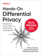
For example, consider X = [1,2,4] and Y = [2, 4, 6]. The numbers 2 and 4 appear in both X and Y, so they are not in the symmetric difference. The number 1 appears in X and not Y, and 6 appears in Y and not X, so they are both in the symmetric difference.
Therefore
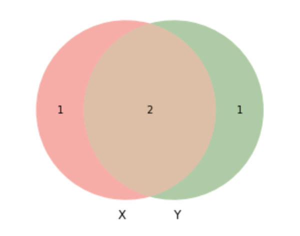
Figure 3-1. Symmetric Difference between databases X and Y is composed of the elements in X and y that are not part of the intersection
- Neighboring (or Adjacent) Databases
-
Two databases
Intuition for Neighboring Databases
Differential privacy formalizes the concept of a privacy guarantee in a data release. To illustrate the privacy guarantees provided by differential privacy, you first need to understand what a privacy violation is. Think of the following scenario: Anna, a data analyst, is doing research that requires querying a database. Barb, is one of the database participants.
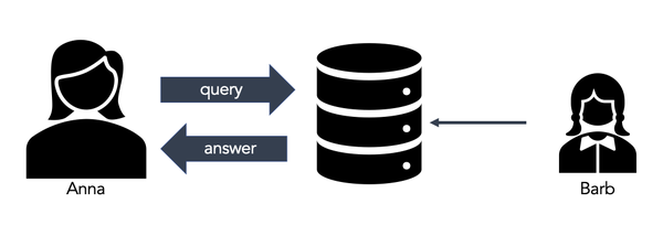
Figure 3-2. One of the individuals in the database is Barb. If Anna learns anything about Barb, that is a privacy violation.
Now suppose Anna does the same research on a neighboring database without Barb’s data. Anna’s research violates Barb’s privacy if her research conclusion changes by querying the neighboring database.
Figure 3-3. If Anna can learn something similar from the same database minus Barb, then there is no privacy violation.
Analogously, if Anna learns something similar from a database without Barb, then there is no privacy violation. Differential Privacy comes from the notion that the presence or absence of any individual in a database should not alter the data analysis results.
Moreover, if the output of a query is differentially private, the presence or absence of Barb (neighboring databases) in the dataset should not significantly change the data analysis result.
Sensitivity
In our classroom example, we defined the local sensitivity of a function as the maximum possible variation in a function’s output when the function is applied to neighboring databases. In other words, the local sensitivity is the greatest amount that a function output can change when computed on an adjacent dataset.
Understanding and computing the sensitivity of a function is important because it quantifies how much a single user can impact the output of a function. The sensitivity will be an important input parameter of differential privacy mechanisms, as it influences how much noise must be added to satisfy a privacy guarantee. One way to express the sensitivity of a function is via the absolute distance metric.
- Absolute Distance
-
The absolute distance measures the absolute value of the difference between two scalars
The absolute distance metric is used in contexts where the output of the function is scalar-valued.
Let
Recall from the definition that
Let’s use the sensitivity definition and calculate the sensitivity of a function.
Given a function
The sensitivity of a function is defined as:
where
According to the definition of neighboring databases, the symmetric distance of
Formalizing the Concept of Differential Privacy
The formalization of differential privacy will help you understand the core concept of privacy loss.
As mentioned in the beginning of this chapter, the idea of a differentially private mechanism is to provide similar outputs given the presence or absence of any individual. Let’s define it in terms of neighboring databases.
- Differential Privacy
-
A mechanism
The definition of
Additionally, the smaller the
The parameter
Achieving Differential Privacy: Mechanisms for Output Perturbation
A differentially private mechanism is a randomized computation that has nearly the same output for adjacent datasets. This is sometimes achieved by adding noise to the result of a query. For the differential privacy guarantee to hold, the query must have bounded sensitivity, and the noise must be sampled from a carefully-calibrated distribution. A differentially private mechanism is a function with a mathematically proven privacy guarantee. The function samples from a carefully-calibrated noise distribution that is more concentrated around the exact value.
As discussed before, differential privacy can be achieved via output perturbation.
This means that adding “random noise” to query results that have bounded sensitivity
can guarantee differentially private protections for individuals in the database.
More formally, to guarantee the privacy of individuals in a database
The random noise should be calibrated to mask the presence or absence of any individual in the database. In other words, any one entry of the database should not affect the output distribution of the algorithm significantly. This means that an adversary, who knows all but one entry in the database, cannot gain significant information about the unknown entry by observing the output of the algorithm.
Note that differential privacy is a characteristic of a query (or more generally, an algorithm). However, throughout this book the term differentially private data release will be used to refer to the output of differentially privacy queries (or algorithms).
As described in chapter 2, the purpose of a differential privacy mechanism is to extract information from a database while hiding the presence or absence of any individual. Differential privacy mechanisms allow data analysts to learn insights from a population while preserving the privacy of individuals.
Example: Returning to the Classroom
Suppose there exist two databases
Using the student dataset, we will define
From the student’s perspective, they should not be able to distinguish if the mechanism was applied to
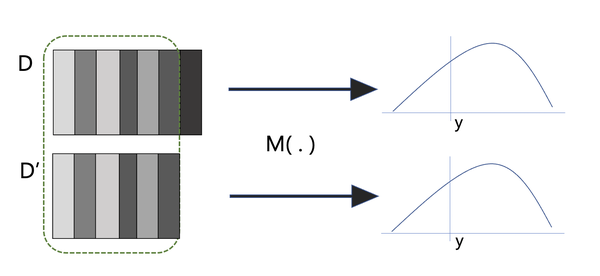
Figure 3-4. Differential Privacy mechanisms applied to neighboring databases should result in indistinguishable results.
Why do we use the concept of two adjacent databases?
The concept of neighboring databases helps rationalize about how much an individual can contribute to the output of a query. This concept will help you understand how to construct a mechanism that will mask the presence or absence of any individual.
Privatizing Numeric Queries: Laplace Mechanism
The Laplace Mechanism provides a way to achieve
The Laplace Mechanism consists of perturbing the output of a numeric function
We will mostly be concerned with the case where
The Laplace mechanism is defined as
where the
The parameters of the Laplace Distribution are crucially important for guaranteeing DP. If the distribution is too thin, then privacy will not be preserved. Similarly, if the distribution is too wide, then too much noise will be added and the statistic will not be useful.
privacy loss parameter:
The second parameter we need to define is the privacy loss parameter
You can think of
Proving the Laplace Mechanism provides
How can you be sure that the Laplace Mechanism guarantees differential privacy? Don’t take our word for it, read through the proof! For each step, try to understand the mathematical reasoning that is happening, and work step-by-step until you arrive at the conclusion.
Implementing Differentially Private Queries with SmartNoise
SmartNoise 3 is a set of tools for creating differentially private reports, dashboards, synopses, and synthetic datasets.
SmartNoise includes a SQL processing library and a synthetic data library. The SQL processing library provides a method to query Spark and other popular database engines. You can also use the library to issue queries against a pandas dataframes.
For most common SQL queries, these are the default mechanisms:
| Query | Default Mechanism |
|---|---|
Count | Geometric Mechanism |
Sum (int) | Geometric Mechanism |
Sum (float) | Laplace Mechanism |
Threshold | Laplace Mechanism |
The SmartNoise SQL library can be installed via pip command:
pipinstallsmartnoise-sql
Example 1: Differentially Private Counts
The SmartNoise library works as a wrapper for the OpenDP Library that simplifies common database queries, such as counts, sums and averages.
SmartNoise requires the trusted curator to load the dataset, specify dataset metadata, and choose the privacy loss parameters. The library automatically calculates the sensitivity based on the dataset metadata and query. Although the library offers default mechanisms for each query type, the user can easily change the desired mechanism.
We will use the student dataset 4 in our examples in this chapter.
importpandasaspddf=pd.read_csv('student.csv')## load the dataset
In order to use the SmartNoise SQL library, you need to specify dataset metadata via a yaml file. The metadata describes the data types of columns, and some additional metadata depending on the data type. For numeric columns, the metadata should include the lower and the upper values in the column. For categorical columns, the metadata should include the cardinality of the categorical variable.
Database:MySchema:MyTable:row_privacy:Trueage:type:intlower:15upper:25G3:type:intlower:0upper:20famsize:cardinality:2type:stringschool:cardinality:2type:stringabsences:type:intlower:0upper:50
To load the data, you need to define three things: the path to the yaml file, a per-query privacy loss parameter, and the pandas dataframe.
Recall that the Laplace mechanism satisfies
>>>fromimportlib.metadataimportmetadata>>>fromsnsql.sql._mechanisms.baseimportMechanism>>>fromsnsqlimportPrivacy>>>fromsnsqlimportfrom_df>>>fromsnsql.sql.privacyimportStat>>>metadata='student.yaml'## load metadata>>>privacy=Privacy(epsilon=1.0)## set privacy loss parameter>>>reader=from_df(df,privacy=privacy,metadata=metadata)## initialize the method from_df to query pandas dataframes
The total privacy loss will increase by
Once the data is initialized by the SmartNoise Library, you can construct queries using SQL syntax to query the dataframe.
You can use ``privacy.mechanisms.map`` to define which differential privacy mechanism to use in the data analysis.
The following executes a count query to get the number of students in the dataframe.
query='SELECT Count(*) AS students FROM MySchema.MyTable'## define the desired queryprivacy.mechanisms.map[Stat.count]=Mechanism.laplace("Running query with Laplace mechanism for count:")(privacy.mechanisms.map[Stat.count])(reader.execute_df(query))
Running query with Laplace mechanism for count:
Mechanism.laplace
   students
0       650
The result of the private count query is 650 students. The same query without privacy preserving mechanisms would return a result of 649 students.
Example 2: Differentially Private Sum
Using the same dataframe from the previous example, you can make other kinds of queries that illustrate how to use SmartNoise. To query the number of absences of all students, you can define a SQL query and run the private analysis as follows:
query='SELECT SUM(absences) AS sum_absences FROM MySchema.MyTable 'privacy.mechanisms.map[Stat.sum_int]=Mechanism.laplace("Running query with Laplace mechanism for count:")(privacy.mechanisms.map[Stat.sum_int])(reader.execute_df(query))
Running query with default mechanisms:
Mechanism.geometric
   sum_absences
0    2192
The result of the private sum is 2192. The data analysis without privacy preserving mechanisms would return a result of 2255.
Consider a scenario where a new student enrolls in the school. If the results from the privatized data analysis is published, and then the analyses are re-published after the new student has enrolled, then due to the use of differential privacy, the number of absences contributed by the new student is kept private.
Composition of Differential Privacy Queries
It is common to release multiple differentially private queries on the same dataset. When releasing more than one query, you must calculate an overall privacy loss based on the privacy loss of each query. In the terminology of differential privacy, the composition of differentially private queries is itself a differentially private query. Take care not to confuse the DP composition with functional composition, where the output of one function is used as the input to another function.
As you would expect, as you increase the number of differentially private queries, the privacy loss increases. There are many variations of composition! The most fundamental is the basic composition, where a set of queries are computed and released together in a single batch. The privacy loss of the basic composition is easy to calculate, as it tends to increase linearly in the number of queries.
- Basic Composition
-
For a batch of
Going back to the classroom example, suppose the teacher decides to release the mean score of the midterm and the final
exams.
If the teacher uses a
A simple relaxation is the sequential composition, which allows you to adaptively choose the next query after releasing the previous query. Interestingly, sequential composition does not assume query independence, which means that privacy guarantees remain intact even when a query incorporates results from previous queries.
- Sequential Composition
-
For a sequence of
An unfortunate drawback to sequential composition is that you must fix the privacy parameters for all future queries before making your first release. If you fix your privacy parameters ahead-of-time, then the sequential composition enjoys the same linear sum behavior as in the basic composition. Privacy odometers relax this requirement, with the downside that they tend to charge a bit more for each query. In many situations, having the flexibility to adaptively choose privacy parameters is worth the tradeoff.
A special case of DP composition is when distinct queries are applied to disjoint subsets of the database. In this case, the privacy loss is not the sum of all the epsilons, but rather is the maximum epsilon. This composition is known as parallel composition.
- Parallel Composition
-
For a sequence of
In the classroom example, suppose the teacher is interested in understanding the mean score of the final exams of two
disjoint subsets of students: group 1 is the students with at least one parent who is a teacher, and group 2 are
students with parents who are not teachers.
If the teacher uses a
Example 4: Multiple Queries from a Single Database
Using the same dataframe from the previous examples, let’s query the average grade for exam 3 (column G3). Now, there are two different partitions of the data: Students whose family size is greater than 3, and students whose family size is less than or equal to 3.
>>>query='SELECT famsize as Family_Size, AVG(G3) AS average_scoreFROMMySchema.MyTableGROUPBYfamsize'>>>("Running query with default mechanisms:")>>>res=reader.execute_df(query)>>>(res)Runningquerywithdefaultmechanisms:Family_Sizeaverage_score0GT311.8250191LE312.018476
Now let’s try another partition of the data: Students from school GP, and students from school MS.
query='SELECT school, AVG(G3) AS average_score FROM MySchema.MyTable GROUP BY school'("Running query with default mechanisms:")(reader.execute_df(query))
Running query with default mechanisms:
  school  average_score
0     GP      12.755956
1     MS      10.721144
Now let’s calculate the privacy loss after the two queries above.
The first query returns the average score for two group of students.
Both queries utilize the Laplace mechanism with privacy loss parameter
The second query also provides the average score for two disjoint groups of students.
Just like the first query, it provides
Finally, the final privacy guarantee can be computed using sequential composition.
Given that we have a sequence of two queries that provides
Post-Processing Immunity
Another important differential privacy property is immunity to post-processing. This means that you can apply transformations to a DP release and know that the result is still differentially private.
Differentially private data releases are immune to Post-processing
Theorem: Let
With an understanding of these definitions and theorems, you are ready to dive into use cases and deeper theories in differential privacy. By now, you should be comfortable answering basic questions about a DP data analysis approach: Does noise from a particular distribution satisfy DP? Is the sensitivity of a mechanism small enough to allow for meaningful noise addition? Is the sensitivity even defined? You should also understand what DP guarantees (and what it doesn’t), and how your epsilon changes the output of your DP data release.
In the next chapter, you will build on your solid foundation in the basics of DP. This chapter will cover notions that generalize adjacency and sensitivity, to scenarios where two datasets can differ by more than a single value. In this case, you will want to answer a more general question: given a change in the input of my analysis, what is maximum change in its output?
Exercises
-
Given X = [1,2,3,4,5,6,7,8,9,10], calculate COUNT(X).
-
Calculate COUNT(Y) for each adjacent dataset Y.
-
Using the previous two results, verify that the sensitivity of COUNT is 1.
-
-
What is the sensitivity (in terms of the absolute distance) of the following functions, where x is a binary array of size n:
-
-
Which privacy loss parameter provides stronger privacy guarantees:
-
Using the SmartNoise Library and the Student dataset, make the following queries:
-
With a privacy loss parameter of
-
With a privacy loss parameter of
-
1 A detailed and formal definition of independent random variables is in appendix A.
2 appendix A
3 smartnoise.org
4 https://archive.ics.uci.edu/ml/datasets/student+performance