
Chapter 13. Putting It All Together: Experimenting and Ranking
In the last few chapters we have covered many aspects of ranking, including different kinds of loss functions as well as metrics for measuring the performance of ranking systems. In this Putting It All Together chapter we will show an example of a ranking loss and ranking metric on the Spotify Million Playlist dataset.
This Putting It All Together chapter is different from the previous ones in the sense that it encourages a lot more experimentation and is more open ended than the previous ones, whose goal was to introduce concepts and infrastructure. This chapter on the other hand is written to encourage you to roll up your sleeves and engage directly with loss functions and writing metrics.
Experimention Tips
Before we begin digging into the data and modelling, let’s cover some practices that will make your life easier when doing a lot of experimentation and rapid iteration. These are general guidelines that we have found that make our experimentation faster. As a result, we’re able to rapidly iterate towards solutions that help us reach our objectives.
Experimental code is different from engineering code in the sesnse that the code is written to explore idea spaces and not for robustness. The goal is to achive maximum velocity while not sacrificing too much in terms of code quality. So some thought might be put in as to whether a piece of code should be thorougly tested or if this isn’t necessary because the code is only present to test a hypothesis and then it will be thrown away. With that in mind here are some tips. Please keep in mind that these tips are the opinion of the authors, developed over time, and are not hard and fast rules, just some flavored opinions that some may disagree with.
Keep it simple
In terms of the overall structure of research code, it’s best to keep it as simple as possible. Try not to overthink too much in terms of inheritance and re-usability during the early stages of the lifecycle of exploration. At the start of a project we usually don’t know what a project needs yet, so the preference should be keeping the code easily readable and simple for debugging. That means you don’t have to focus too much on code re-use because at the early stage of a project there will be many code changes while the structure of the model, data ingestion and interaction of different parts of a system are being worked out. When the uncertainties have been worked out, then you can re-write the code into a more robust form, but it actually slows down velocity to refactor too early. A general rule of thumb is that it is ok to copy code three times, and then refactor out into a library the fourth time, because one has seen enough use cases to justify the reuse of code. If refactoring is done too early, you might not have seen enough use cases of a piece of code to cover the possible use cases that it might need to handle.
Debugging print statements
If you’ve read a number of research papers on machine learning, you may expect the data to be fairly clean and orderly at the start of a project. However, real world data can be messy, with missing fields and unexpected values. Having lots of print functions to print a sample of the data allows one to visually inspect a sample of the data and it also helps in crafting the input data pipelines and transformations of the data to feed the model. Also, printing sample outputs of the model is useful in making sure the output is as expected. The most important places to include logging are the input and output schema between components of your system; these help understand where reality may be deviating from expecations. Later, you can make unit tests to ensure that refactoring of the model doesn’t break anything, but the unit tests can wait for when the model architecture is stable. A good rule of thumb is to add unit tests when you want to refactor code or reuse or optimize the code to preserve functionality or when the code is stable and you want to ensure that it doesn’t break a build. Another good use case of adding print statements is when you inevitably run into NaNs, or Not a Number, errors when running training code.
In Jax, one can enable NaN debugging using the following lines
fromjaximportconfigconfig.update("jax_debug_nans",True)@jax.jitdeff(x):jax.debug.("Debugging{x}",x=x)
The debug NaNs configuration setting will re-run a jitted function if it finds any NaNs and the debug print will print the value of the tensors even inside a JIT. A regular print won’t work inside a JIT because it is not a compilable command and is skipped over during the tracing, so you have to use the debug print function instead, which does work inside a JIT.
Optimization
In research code, there is a lot of temptation to optimize early; in particular focusing on the implementation of your models or system to ensure they’re effecient computationally or the code is elegant. However, research code is written for higher velocity in experimentation not execution speed. Our suggestion is do not optimize too early unless it hinders research velocity. One reason for this is the system might not be complete, so optimizing one part might not make sense if another part of the system is even slower and is the actual bottleneck. Another reason is the part that you are optimizing might not make it to the final model, so all the optimization work might go to waste if the code is refactored away anyway. Finally, optimization might actually hinder the ability to modify or inject newer design choices in terms of architecture or functionality. Optimized code tends to have certain choices that were made that fit the current structure of the data flow but might not be amenable to futher changes. For example, in the code for this chapter one possible optimization choice would have been to batch together playlists of the same size so that the code might be able to run in larger batches. However, at this point of the experimentation, it would have been a premature optimization and distract because it might make the metrics code more complicated. Our gentle advice would be to defer optimization until after the bulk of experimentation has been done and the archicture, loss functions, and metrics have been chosen and settled upon.
Keeping track of changes
In research code, there are probably too many variables at play for you to change them one at a time to see what the effects are. This problem is particularly noticeable in the case of larger data sets where it takes a lot of runs to determine what change causes what effects. So in general it is still a good idea to fix a number of parameters and change the code bit by bit so that you are able to keep track of the change that causes the most improvement. Parameters have to be tracked but so does the code changes. One way to keep track of changes is through services such as Weights and Biases that we have discussed before Chapter 5. It is a good idea to keep track of the exact code that led to a change and the parameters so that experiments can be reproduced and analyzed. Especially with research code that changes so frequently and is sometimes not checked in, one has to be diligent in keeping a copy of the code that produced a run somewhere and MLOps tools allow you to track code and hyperparameters.
Feature Engineering
Unlike in academic papers, most applied research is interested in a good outcome rather than a theoretically beautiful result. This means we’re not shackled by purist views that the model has to learn everything about the data by itself. Instead, we’re pragmatic and concerned about good outcomes. We should not discard practices like feature engineering especially when we have very little data or we are crunched for time and need decent results fast. Feature engineering means if you know if some hand crafted feature is correlated positvely or negatively with an outcome like the ranking of an item, then by all means add these engineered features to the data. An example in recommender systems, is if some attribute of the item being scored matches something in the user’s profile. So, if an item has the same artist or album in the user’s playlist, we can return a boolean True, otherwise we return False. This extra feature simply helps the model converge faster and the model can still use other latent features such as embeddings to compensate if the hand engineered features don’t do so well. It is generally a good practice to ablate the hand engineered features once in a while. To do this, hold back an experiment without some features to see if those features have become obsolete over time or if they still benefit the business metrics.
Ablation
Ablation in ML applications is the idea of measuring the change in performance of a model when a particular feature is removed. In computer vision applications, ablation often refers to blocking part of the image or viewfield to see how it impacts the model’s ability to identify or segment things. In other kinds of ML, it can mean to strategically remove certain features.
One gotcha with ablation, is what to replace the feature with. If you simply zero out the feature, that can significantly skew the output of the model. This is called zero-ablation, and can force the model to treat that feature out-of-distribution, which yields less believable outcomes. Instead, some advocate for mean-ablation, or taking the average or most common value of that feature. This allows the model to see values much more expected, and reduce these risks. However, this fails to consider the most important aspects of the kinds of models we’ve been working on – latent high-order interactions. One of the authors has investigated a deeper approach to ablation called causal scrubbing in which you fix the ablation value to be sampled from the posterior distribution produced by other feature values, i.e. a value that “makes sense” with the rest of the values the model will see at that time.
Metrics vs Business Metrics
Sometimes, as machine learning practitioners, we obsess over the best possible metrics our models can achieve. However, we should temper that enthusiam as the best machine learning metric might not totally represent the business interests at hand. Furthermore, other systems that contain business logic might sit on top of our models and modify the output. As a result, it is best not to obsess too heavily over machine learning metrics and to do proper A/B tests that contain business metrics instead since that’s the main measure of a good outcome with machine learning.
The best possible circumstance is to find a loss function which well aligns, or predicts the relvant business metric. This unfortunately is often not easy to find; especially when the business metrics are nuanced or have competing priorities.
Rapid iteration
Don’t be afraid to look at results of runs that are rather short. There’s no need to do a full pass over the data at the beginning when you are figuring out the interaction between a model architecture and the data. It’s ok to do some rapid runs with minor tweaks to see how they change the metrics over a short number of time steps. In the Spotify million playlist data set, we tweaked the model architecture using 100k playlists before doing longer runs. Sometimes the changes can be so dramatic that the effects can be seen immediately even at the first test set evaluation.
Now that we have the basics of experimental research coding covered let’s now hop over to the data and code and play a bit with modelling music recommendations.
Spotify Million Playlist Dataset
The code for this section can be found in this book’s Github repo. The documentation for the data can be found at Spotify Million Playlist Dataset Challenge.
The first thing we should do is take a look at the data with
lessdata/spotify_million_playlist_dataset/data/mpd.slice.0-999.json
It should produce the following output:
{"info":{"generated_on":"2017-12-03 08:41:42.057563","slice":"0-999","version":"v1"},"playlists":[{"name":"Throwbacks","collaborative":"false","pid":0,"modified_at":1493424000,"num_tracks":52,"num_albums":47,"num_followers":1,"tracks":[{"pos":0,"artist_name":"Missy Elliott","track_uri":"spotify:track:0UaMYEvWZi0ZqiDOoHU3YI","artist_uri":"spotify:artist:2wIVse2owClT7go1WT98tk","track_name":"Lose Control (feat. Ciara & Fat Man Scoop)","album_uri":"spotify:album:6vV5UrXcfyQD1wu4Qo2I9K","duration_ms":226863,"album_name":"The Cookbook"},}}
When encountering a new data set, it is always important to look at the dataset and plan what features to use to generate recommendations for the data. One possible goal of the Spotify Million Playlist Dataset Challenge is to see if the next tracks in a playlist can be predicted from the first 5 tracks in the playlist. In this case, we have several features that might be useful for the task. There are track, artist and album Universal Resource Identifiers (URIs) which are unique identifiers for tracks, artists and albums respectively. And there are artist and album names and names of playlists. There are also numerical features like duration of a track and the number of followers in a playlist. Intuitively, the number of followers of a playlist should not affect the ordering of tracks in a playlist so you might want to look for better features before using these possibly uninformative features. Looking at the overall statistics of features one can also obtain a lot of insight:
lessdata/spotify_million_playlist_dataset/stats.txtnumberofplaylists1000000numberoftracks66346428numberofuniquetracks2262292numberofuniquealbums734684numberofuniqueartists295860numberofuniquetitles92944numberofplaylistswithdescriptions18760numberofuniquenormalizedtitles17381avgplaylistlength66.346428topplaylisttitles10000country10000chill8493rap8481workout8146oldies8015christmas6848rock6157party5883throwback5063jams5052worship4907summer4677feels4612new4186disney4124lit4030throwbacks
First of all, notice that the number of tracks is more than the number of playlists. So this implies that there might be quite a few tracks with very little training data. So the track_uri might not be a feature that generalizes very well. On the other hand, the album_uri and artist_uri would generalize because they would occur multiple times in different playlists. For the sake of code clarity we will mostly work with the the album_uri and artist_uri as the features that represent a track. In previous Putting It All Together chapters, we have demonstrated the use of content based features or text token based features that may be used instead, but direct embedding features are the clearest to demonstrate ranking on. In a real world application embedding features and content based features may be concatenated together to form a feature that generalizes better for recommendation ranking. For the purposes of this chapter, we will represent a track as the tuple of (track_id, album_id, artist_id) where the id is an integer representing the URI. We will build dictionaries that map from the URI to the integer id in the next section.
Building URI dictionaries
Similarly to the Putting It All Together:Data Processing and Counting Recommender Chapter 8 we will first start by constructing a dictionary for all the URIs. This dictionary allows us to represent the text URI as an integer for faster processing on the Jax side as we can easily look up embeddings from integers as opposed to arbitrary URI strings.
Here is the code for make_dictionary.py
importglobimportjsonimportosfromtypingimportAny,Dict,TuplefromabslimportappfromabslimportflagsfromabslimportloggingimportnumpyasnpimporttensorflowastfFLAGS=flags.FLAGS_PLAYLISTS=flags.DEFINE_string("playlists",None,"Playlist json glob.")_OUTPUT_PATH=flags.DEFINE_string("output","data","Output path.")# Required flag.flags.mark_flag_as_required("playlists")defupdate_dict(dict:Dict[Any,int],item:Any):"""Adds an item to a dictionary."""ifitemnotindict:index=len(dict)dict[item]=indexdefdump_dict(dict:Dict[str,str],name:str):"""Dumps a dictionary as json."""fname=os.path.join(_OUTPUT_PATH.value,name)withopen(fname,"w")asf:json.dump(dict,f)defmain(argv):"""Main function."""delargv# Unused.tf.config.set_visible_devices([],'GPU')tf.compat.v1.enable_eager_execution()playlist_files=glob.glob(_PLAYLISTS.value)track_uri_dict={}artist_uri_dict={}album_uri_dict={}forplaylist_fileinplaylist_files:("Processing ",playlist_file)withopen(playlist_file,"r")asfile:data=json.load(file)playlists=data["playlists"]forplaylistinplaylists:tracks=playlist["tracks"]fortrackintracks:update_dict(track_uri_dict,track["track_uri"])update_dict(artist_uri_dict,track["artist_uri"])update_dict(album_uri_dict,track["album_uri"])dump_dict(track_uri_dict,"track_uri_dict.json")dump_dict(artist_uri_dict,"artist_uri_dict.json")dump_dict(album_uri_dict,"album_uri_dict.json")if__name__=="__main__":app.run(main)
Whenever a new URI is encountered we simply increment a counter and assign that unique identifier to the URI. We do this for tracks, artists and albums and save it as a json file. Although we could have used a data processing framework like pyspark for this, it is important to take note of the data size. If the data size is small, like a million playlists, it would just be faster to do it on a single machine. One should be wise about when to use a big data processing framework, and for small data sets it can sometimes be faster to simply run the code on one machine instead of writing code that runs on a cluster.
Building the Training Data
Now that we have the dictionaries, we can use them to convert the raw JSON playlist logs into a more usable form for machine learning training. The code for this is make_training.py.
importglobimportjsonimportosfromtypingimportAny,Dict,Tuplefromabslimportappfromabslimportflagsfromabslimportloggingimportnumpyasnpimporttensorflowastfimportinput_pipelineFLAGS=flags.FLAGS_PLAYLISTS=flags.DEFINE_string("playlists",None,"Playlist json glob.")_DICTIONARY_PATH=flags.DEFINE_string("dictionaries","data/dictionaries","Dictionary path.")_OUTPUT_PATH=flags.DEFINE_string("output","data/training","Output path.")_TOP_K=flags.DEFINE_integer("topk",5,"Top K tracks to use as context.")_MIN_NEXT=flags.DEFINE_integer("min_next",10,"Min number of tracks.")# Required flag.flags.mark_flag_as_required("playlists")defmain(argv):"""Main function."""delargv# Unused.tf.config.set_visible_devices([],'GPU')tf.compat.v1.enable_eager_execution()playlist_files=glob.glob(_PLAYLISTS.value)track_uri_dict=input_pipeline.load_dict(_DICTIONARY_PATH.value,"track_uri_dict.json")("%dtracks loaded"%len(track_uri_dict))artist_uri_dict=input_pipeline.load_dict(_DICTIONARY_PATH.value,"artist_uri_dict.json")("%dartists loaded"%len(artist_uri_dict))album_uri_dict=input_pipeline.load_dict(_DICTIONARY_PATH.value,"album_uri_dict.json")("%dalbums loaded"%len(album_uri_dict))topk=_TOP_K.valuemin_next=_MIN_NEXT.value("Filtering out playlists with less than%dtracks"%min_next)raw_tracks={}forpidx,playlist_fileinenumerate(playlist_files):("Processing ",playlist_file)withopen(playlist_file,"r")asfile:data=json.load(file)playlists=data["playlists"]tfrecord_name=os.path.join(_OUTPUT_PATH.value,"%05d.tfrecord"%pidx)withtf.io.TFRecordWriter(tfrecord_name)asfile_writer:forplaylistinplaylists:ifplaylist["num_tracks"]<min_next:continuetracks=playlist["tracks"]# The first topk tracks are all for the context.track_context=[]artist_context=[]album_context=[]# The rest are for predicting.next_track=[]next_artist=[]next_album=[]fortidx,trackinenumerate(tracks):track_uri_idx=track_uri_dict[track["track_uri"]]artist_uri_idx=artist_uri_dict[track["artist_uri"]]album_uri_idx=album_uri_dict[track["album_uri"]]iftrack_uri_idxnotinraw_tracks:raw_tracks[track_uri_idx]=trackiftidx<topk:track_context.append(track_uri_idx)artist_context.append(artist_uri_idx)album_context.append(album_uri_idx)else:next_track.append(track_uri_idx)next_artist.append(artist_uri_idx)next_album.append(album_uri_idx)assert(len(next_track)>0)assert(len(next_artist)>0)assert(len(next_album)>0)record=tf.train.Example(features=tf.train.Features(feature={"track_context":tf.train.Feature(int64_list=tf.train.Int64List(value=track_context)),"album_context":tf.train.Feature(int64_list=tf.train.Int64List(value=album_context)),"artist_context":tf.train.Feature(int64_list=tf.train.Int64List(value=artist_context)),"next_track":tf.train.Feature(int64_list=tf.train.Int64List(value=next_track)),"next_album":tf.train.Feature(int64_list=tf.train.Int64List(value=next_album)),"next_artist":tf.train.Feature(int64_list=tf.train.Int64List(value=next_artist)),}))record_bytes=record.SerializeToString()file_writer.write(record_bytes)filename=os.path.join(_OUTPUT_PATH.value,"all_tracks.json")withopen(filename,"w")asf:json.dump(raw_tracks,f)if__name__=="__main__":app.run(main)
The code here reads in a raw playlist JSON file, converts the URIs from textual identifiers to the index in the dictionary, and also filters out playlists that are under a minimum size. In addition, we partition the playlist such that the first five elements are grouped into the context, or user that we are recommending items for, and next items, which are the items we wish to predict for a given user. We call the first five elements the context because it is the group of features that represent a playlist and there might not be a one to one mapping between a playlist and a user because a user might have more than one playlist. We then write each playlist as a Tensorflow Example in a Tensorflow Record file for use with the Tensorflor data input pipeline. The records will always contain five tracks, albums and artists for the context and at least five more next tracks for learning the prediction tasks of predicting the next tracks.
Note
The reason we use TensorFlow objects here is how compatible they are with JAX, while introducing some very convenience data formats.
We also store unique rows of tracks with all the features which is mostly for debugging and display should we need to convert a track_uri into a human readable form. This track data is stored in all_tracks.json.
Reading the Input
The input is then read via input_pipeline.py
importglobimportjsonimportosfromtypingimportSequence,Tuple,Setimporttensorflowastfimportjax.numpyasjnp_schema={"track_context":tf.io.FixedLenFeature([5],dtype=tf.int64),"album_context":tf.io.FixedLenFeature([5],dtype=tf.int64),"artist_context":tf.io.FixedLenFeature([5],dtype=tf.int64),"next_track":tf.io.VarLenFeature(dtype=tf.int64),"next_album":tf.io.VarLenFeature(dtype=tf.int64),"next_artist":tf.io.VarLenFeature(dtype=tf.int64),}def_decode_fn(record_bytes):result=tf.io.parse_single_example(record_bytes,_schema)forkeyin_schema.keys():ifkey.startswith("next"):result[key]=tf.sparse.to_dense(result[key])returnresultdefcreate_dataset(pattern:str):"""Creates a spotify dataset.Args:pattern: glob pattern of tfrecords."""filenames=glob.glob(pattern)ds=tf.data.TFRecordDataset(filenames)ds=ds.map(_decode_fn)returnds
We use Tensorflow data’s functionality to read and decode the Tensorflow Records and Examples. For that to work we need to supply a schema, or a dictionary, telling the decoder what names and types of features to expect. Since we have picked five tracks each for the context, we should expect five each of track_context, album_context and artist_context. However, since the playlists themselves are of variable lengths, we tell the decoder to expect variable length integers for the next_track, next_album and next_artist features.
The second part of input_pipeline.py is for re-usable input code to load the dictionaries and track metadata.
defload_dict(dictionary_path:str,name:str):"""Loads a dictionary."""filename=os.path.join(dictionary_path,name)withopen(filename,"r")asf:returnjson.load(f)defload_all_tracks(all_tracks_file:str,track_uri_dict,album_uri_dict,artist_uri_dict):"""Loads all tracks."""withopen(all_tracks_file,"r")asf:all_tracks_json=json.load(f)all_tracks_dict={int(k):vfork,vinall_tracks_json.items()}all_tracks_features={k:(track_uri_dict[v["track_uri"]],album_uri_dict[v["album_uri"]],artist_uri_dict[v["artist_uri"]])fork,vinall_tracks_dict.items()}returnall_tracks_dict,all_tracks_featuresdefmake_all_tracks_numpy(all_tracks_features):"""Makes the entire corpus available for scoring."""all_tracks=[]all_albums=[]all_artists=[]items=sorted(all_tracks_features.items())forrowinitems:k,v=rowall_tracks.append(v[0])all_albums.append(v[1])all_artists.append(v[2])all_tracks=jnp.array(all_tracks,dtype=jnp.int32)all_albums=jnp.array(all_albums,dtype=jnp.int32)all_artists=jnp.array(all_artists,dtype=jnp.int32)returnall_tracks,all_albums,all_artists
We also supply a utility function to convert the all_tracks.json file into the entire corpus of tracks for scoring in the final recommendations. After all, the goal is to rank the entire corpus given the first five context tracks and see how well they match the given next track data.
Modelling the problem
Next, let’s think of how we will model the problem. We have five context tracks, each with an associated artist and album. We know that we have more tracks than playlists, so for now we will simply ignore the track_id and just use the album_id and artist_id as features. One strategy could be to use one hot encoding for the album and artist, and this would work well, but one hot encoding tends to lead to models with high precision but less generalization. An alternate way to represent identifiers is to embed them. That is, to make a look up table to an embedding of a fixed size that is lower dimensional that the cardinality of the identifiers. This embedding can be thought of as a low rank approximation to the full rank matrix of identifiers. We covered the concept of low rank embeddings in earlier chapters and we use that concept here as features to represent the album and artists.
Take a look at models.py which contains the code for the SpotifyModel.
fromfunctoolsimportpartialfromtypingimportAny,Callable,Sequence,Tuplefromflaximportlinenasnnimportjax.numpyasjnpclassSpotifyModel(nn.Module):"""Spotify model that takes a context and predicts the next tracks."""feature_size:intdefsetup(self):# There are too many tracks and albums so limit to this number by hashing.self.max_albums=100000self.album_embed=nn.Embed(self.max_albums,self.feature_size)self.artist_embed=nn.Embed(295861,self.feature_size)defget_embeddings(self,album,artist):"""Given track, album, artist indices return the embeddings.Args:album: ints of shape nx1artist: ints of shape nx1Returns:Embeddings representing the track."""album_modded=jnp.mod(album,self.max_albums)album_embed=self.album_embed(album_modded)artist_embed=self.artist_embed(artist)result=jnp.concatenate([album_embed,artist_embed],axis=-1)returnresult
In the setup code, notice that we have two different embeddings for the albums and the artists. There are a lot of albums so we show one way to reduce the memory footprint of album embeddings and that is to take the mod of a smaller number than the number of embeddings so that multiple albums might share an embedding. If more memory is available you can remove the mod, but this technique is demonstrated here as a way of getting some benefit of having an embedding for a feature with very large cardinality.
The artist is probably the most informative feature and there are far fewer unique artists, so we have a one to one mapping between the artist_id and the embeddings. When we convert the tuple of (album_id, artist_id) to an embedding, we do separate lookups for each id and then concatenate the embeddings and return one complete embedding to represent a track. If more playlist data becomes available, then you might also want to embed the track_id. However, given that there are more unique tracks than playlists, the track_id feature would not generalize well until we have more playlist data so that the track_id occurs more often as observations. A general rule of thumb is that a feature should occur at least 100 times to be useful, otherwise the gradients for that feature will not be updated very often and it might as well be a random number because it is initialized as such.
In the call section we do the heavy lifting of computing the affinity of a context to other tracks.
def__call__(self,track_context,album_context,artist_context,next_track,next_album,next_artist,neg_track,neg_album,neg_artist):"""Returns the affinity score to the context.Args:track_context: ints of shape nalbum_context: ints of shape nartist_context: ints of shape nnext_track: int of shape mnext_album: int of shape mnext_artist: int of shape mneg_track: int of shape oneg_album: int of shape oneg_artist: int of shape oReturns:pos_affinity: affinity of context to the next track of shape m.neg_affinity: affinity of context to the neg tracks of shape o."""context_embed=self.get_embeddings(album_context,artist_context)next_embed=self.get_embeddings(next_album,next_artist)neg_embed=self.get_embeddings(neg_album,neg_artist)# The affinity of the context to the other track is simply the dot product of# each context embedding with the other track's embedding.# We also add a small boost if the album or artist match.pos_affinity=jnp.max(jnp.dot(next_embed,context_embed.T),axis=-1)pos_affinity=pos_affinity+0.1*jnp.isin(next_album,album_context)pos_affinity=pos_affinity+0.1*jnp.isin(next_artist,artist_context)neg_affinity=jnp.max(jnp.dot(neg_embed,context_embed.T),axis=-1)neg_affinity=neg_affinity+0.1*jnp.isin(neg_album,album_context)neg_affinity=neg_affinity+0.1*jnp.isin(neg_artist,artist_context)all_embeddings=jnp.concatenate([context_embed,next_embed,neg_embed],axis=-2)all_embeddings_l2=jnp.sqrt(jnp.sum(jnp.square(all_embeddings),axis=-1))context_self_affinity=jnp.dot(jnp.flip(context_embed,axis=-2),context_embed.T)next_self_affinity=jnp.dot(jnp.flip(next_embed,axis=-2),next_embed.T)neg_self_affinity=jnp.dot(jnp.flip(neg_embed,axis=-2),neg_embed.T)return(pos_affinity,neg_affinity,context_self_affinity,next_self_affinity,neg_self_affinity,all_embeddings_l2)
Let us dig into this a bit since this is the core of the model code. The first part is pretty straightforward — we convert the indices into embeddings by looking up the album and artist embedding and concatenating them together as a single vector per track. It is in this location that you would add in other dense features by concatenation, or convert sparse features to embeddings as we have done.
The next part computes the affinity of the context to the next tracks. Recall that the context is composed of the first five tracks and the next tracks is the rest of the playlist to be computed. We have several choices here for how we want to represent the context and how to compute the affinity. For the affinity of the context we have chosen the simplest form of affinity, that of a dot product. The other thing to consider is how we treat the context since it is composed of five tracks. One possible way is to average all the context embeddings and use the average as the representation for the context. Another way is to find the track with the maximal affinity as the closest track in the context to that of the next track. Details on various options can be found in Affinity Weighted Embedding. We have found that if a user has diverse interests, finding the max affinity doesn’t update the context embeddings in the same direction as the next track as using the mean embedding does. In the case of playlists, the mean context embedding vector should function just as well because playlists tend to be on a single theme.
Notice that we compute the affinity for the negative tracks as well. This is because we want the next tracks to have more affinity to the context than the negative tracks. In addition to the affinity of the context and next tracks to the context we also compute the L2 norm of the vectors used as a way to regularize the model so it does not overfit on the training data. We also reverse the embedding vectors and compute what we call self-affinity, or the affinity of the context, next and negative embeddings to themselves simply by reversing the list of vectors and taking the dot product. Note that this does not exhaustively compute all the affinities of the set with itself, this again is left as an exercise to the reader as it builds intuition and skill in using Jax.
The results are then returned as a tuple to the caller.
Loss Function
Now, let’s look at train_spotify.py. We will skip the boilerplate code and just look at the evaluation and training steps.
defeval_step(state,y,all_tracks,all_albums,all_artists):result=state.apply_fn(state.params,y["track_context"],y["album_context"],y["artist_context"],y["next_track"],y["next_album"],y["next_artist"],all_tracks,all_albums,all_artists)all_affinity=result[1]top_k_scores,top_k_indices=jax.lax.top_k(all_affinity,500)top_tracks=all_tracks[top_k_indices]top_artists=all_artists[top_k_indices]top_tracks_count=jnp.sum(jnp.isin(top_tracks,y["next_track"])).astype(jnp.float32)top_artists_count=jnp.sum(jnp.isin(top_artists,y["next_artist"])).astype(jnp.float32)top_tracks_recall=top_tracks_count/y["next_track"].shape[0]top_artists_recall=top_artists_count/y["next_artist"].shape[0]metrics=jnp.stack([top_tracks_recall,top_artists_recall])returnmetrics
The first piece of code is the evaluation step. In order to compute the affinities of the entire corpus, we pass in the album and artist indices for every possible track in the corpus to the model and then sort them using jax.lax.top_k. The first two lines are the scoring code for recommending the next tracks from the context during recommendations. LAX is a utility library that comes with Jax that contains functions outside of the numpy API that are handy to work with vector processors like GPUs and TPUs. In the Spotify Million Playlist Dataset Challenge one of the metrics is the recall at top k at the artist and track level. For the tracks, the isin function returns the correct metric of the interesection of the next tracks and the top 500 scoring tracks of the corpus divided by the size of the set of next tracks. This is because the tracks are unique in the corpus. However, Jax’s isin doesn’t support making the elements unique, so for the artist recall metric, we might count artists in the recall set more than once. For the sake of computational efficiency, we use the multiple counts instead so that the evaluation might be computed quickly on the GPU so as not to stall the training pipeline. However, on a final evaluation one might want to move the dataset to CPU for a more accurate metric.
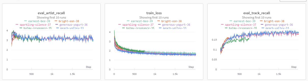
Figure 13-1. Weights and Biases Experiment Tracking
We use Weights and Biases again to track all the metrics and depicted in Figure 13-1 you can see how they fair with each other over several different experiments.
Next, we will look at the loss functions, another juicy part that you can experiment with in the exercises at the end of the chapter.
deftrain_step(state,x,regularization):defloss_fn(params):result=state.apply_fn(params,x["track_context"],x["album_context"],x["artist_context"],x["next_track"],x["next_album"],x["next_artist"],x["neg_track"],x["neg_album"],x["neg_artist"])pos_affinity=result[0]neg_affinity=result[1]context_self_affinity=result[2]next_self_affinity=result[3]neg_self_affinity=result[4]all_embeddings_l2=result[5]mean_neg_affinity=jnp.mean(neg_affinity)mean_pos_affinity=jnp.mean(pos_affinity)mean_triplet_loss=nn.relu(1.0+mean_neg_affinity-mean_pos_affinity)max_neg_affinity=jnp.max(neg_affinity)min_pos_affinity=jnp.min(pos_affinity)extremal_triplet_loss=nn.relu(1.0+max_neg_affinity-min_pos_affinity)context_self_affinity_loss=jnp.mean(nn.relu(0.5-context_self_affinity))next_self_affinity_loss=jnp.mean(nn.relu(0.5-next_self_affinity))neg_self_affinity_loss=jnp.mean(nn.relu(neg_self_affinity))reg_loss=jnp.sum(nn.relu(all_embeddings_l2-regularization))loss=(extremal_triplet_loss+mean_triplet_loss+reg_loss+context_self_affinity_loss+next_self_affinity_loss+neg_self_affinity_loss)returnlossgrad_fn=jax.value_and_grad(loss_fn)loss,grads=grad_fn(state.params)new_state=state.apply_gradients(grads=grads)returnnew_state,loss
There are several losses here, some directly related to the main task, and others are there to help in regularization and generalization.
We initially started with the mean_triplet_loss which is simply a loss that states that the positive affinity, or the affinity of the context tracks to the next tracks, should be one more than the negative affinity, or the affinity of the context tracks to the negative tracks. We will discuss how we experimented to obtain the other auxiliary loss functions.
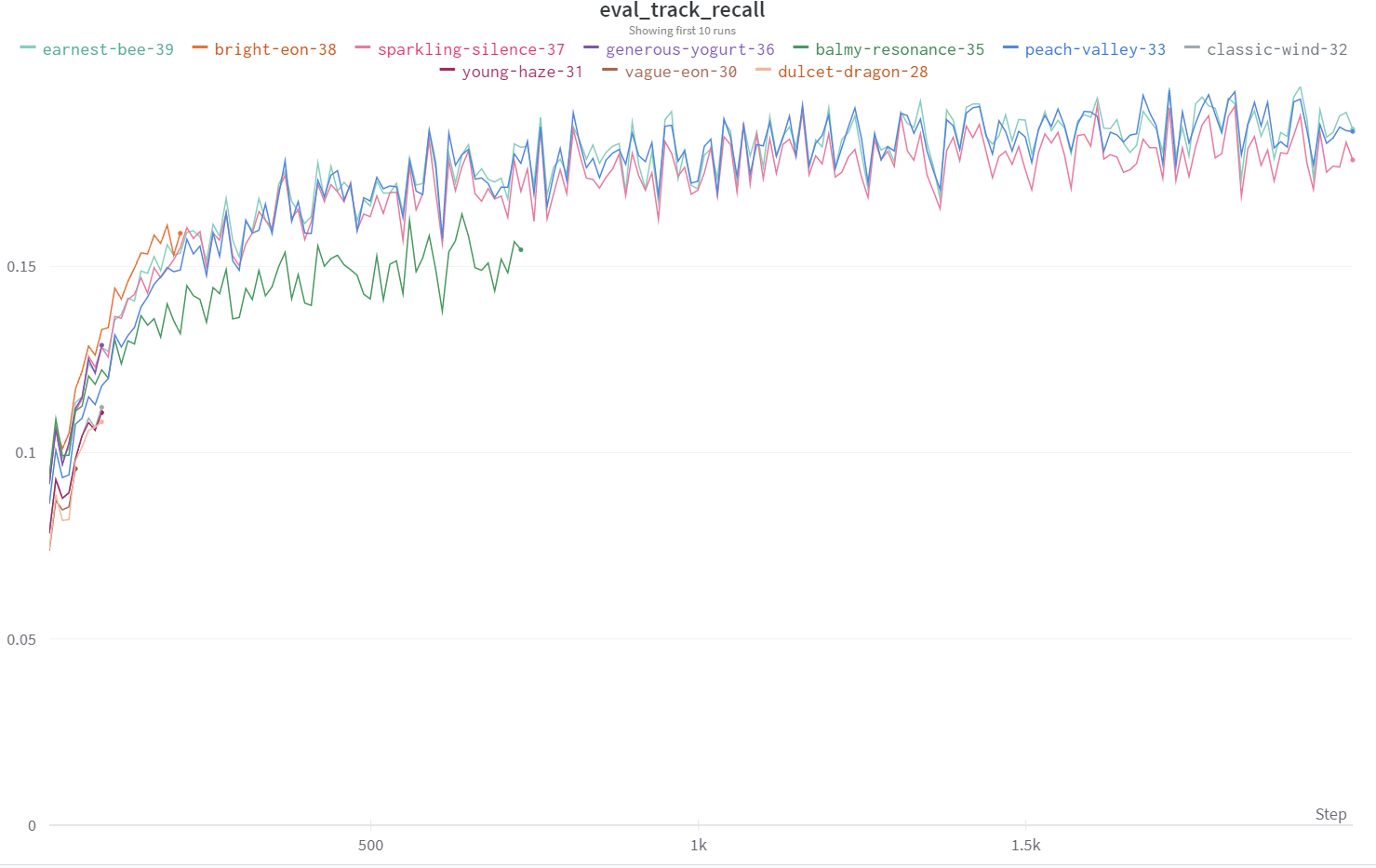
Figure 13-2. Track Recall Experiments
Experiment tracking, depicted in Figure 13-2, is very important in the process of improving the model as is reproducability. We have tried as much as possible to make the training process deterministic by using random number generators from Jax that are reproducable by using the same starting random number generator seed.
We started with the mean_triplet_loss and reg_loss which is the regularization loss as a good baseline. These two losses simply make sure that the mean positive affinity of the context to the next track is one more than the negative affinity of the context to the negative tracks and that the L2 norm of the embeddings do not exceed the regularization thresholds. These correspond to the metrics that did the worst. Notice that we do not run the experiment for the entire data set. This is because for rapid iteration it might be faster to just run on a smaller number of steps first and compare before interleaving occasionally with longer runs that use the entire data set.
The next loss we added was the max_neg_affinity and the min_pos_affinity. This loss was inspired in part by the papers Efficient coordinate descent for ranking with domination loss and Learning to Rank Recommendations
with the k-Order Statistic Loss. However, we do not use the entire negative set but merely a subsample. Why? Because the negative set is noisy. Just because a user hasn’t added a particular track to a playlist doesn’t mean that the track is not relevant to the playlist. It might also be the case that the user hasn’t heard the track yet, so there is some noise due to lack of exposure. We also do not do the sampling step as discussed in the K-order statistic loss paper because sampling is CPU friendly but not GPU friendly. So we combine ideas from both papers and take the largest negative affinity and make it one less than the smallest positive affinity. The addition of this loss on the extremal tracks from both the next and negative sets gave us the next boost in performance in our experiments.
Finally we added the self-affinity losses. These ensure that tracks from the context and next track sets have affinities of at least 0.5 and that the negative track affinities are at most 0. These are dot product affinities and are more absolute as opposed to the relative positive and negative affinities that make the positive affinity one more than the negative affinities. In the end they didn’t help much in the long run but they did help the model converge faster in the beginning. We left it in because on the last training step it still does offer some improvement on the evaluation metrics.
Discussion
This wraps up the explanatory part of this Putting It All Together chapter. Now comes the fun part, the exercises! The reason we offer a lot of exercises is that playing with the data and code is helpful in building out your intuition about different loss functions and ways of modelling the user. Also, thinking about how to write the code allows one to improve in their proficiency at using Jax. So we have a list of helpful exercises to try out that are fun and will help in understanding the material provided in this book.
Exercises
To wrap up this chapter, here are some interesting exercises to experiment with. Doing them should give you lots of intuition about loss functions, the way Jax works and a feel of the experimental process.
Some easy exercises to start with are:
-
Try out different optimizers, e.g. adam, rmsprop
-
Try changing the feature sizes
-
Add in duration as a feature (take care on normalization!)
-
What if you use cosine distance for inference and dot product for training
-
Add in a new metric like Normalized Discounted Cumulative Gain
-
Play with distribution of positive vs negative affinities in the loss
-
Hinge loss with the lowest next track and the highest negative track
Continue exploring with more difficult exercises:
-
Try using the track names as features and see if they help generalize
-
What happens if you use a 2 layer network for affinity?
-
What happens if you use an LSTM to compute affinity?
-
Replace track embeddings with correlation
-
Compute all the self affinities in a set
Summary
What does it mean to replace an embedding with a feature? In our example of positive and negative affinity we used the dot product to compute the affinity between two entities, such as two different tracks, x and y. Rather than having the features as latent, represented by embeddings, an alternative is to manually construct features that represent the affinity between the two entities, x and y. As covered in previous chapters, this can be log counts or Dice correlation coefficient or mutual information. Some kind of counting feature can be made and then stored in a database. Upon training and inference, the database is looked up for each entity x and y and the affinity scores are then used instead of or in conjunction with the dot product that is being learnt. These features tend to be more precise but have less recall than an embedding representation. The embedding representation being of low rank has the ability to generalize better and improve recall. Having counting features is synergistic with embedding features because then one is able to simultaneously improve precision with the use of precise counting features and at the same time improve recall with the help of low rank features like embeddings.
For computing all n^2 affinities of tracks to other tracks in a set consider using Jax’s vmap function. vmap can be used to convert code that for example computes one track’s affinity with all the other tracks and make it run for all tracks vs all other tracks.
We hope that you have enjoyed playing with the data and code and your skill in writing recommender systems in Jax has improved considerably after trying these exercises!