
Ordered and Quantum Treemaps: Making Effective Use of 2D Space to Display Hierarchies
Treemaps, a space-filling method for visualizing large hierarchical data sets, are receiving increasing attention. Several algorithms have been previously proposed to create more useful displays by controlling the aspect ratios of the rectangles that make up a treemap. While these algorithms do improve visibility of small items in a single layout, they introduce instability over time in the display of dynamically changing data, fail to preserve order of the underlying data, and create layouts that are difficult to visually search. In addition, continuous treemap algorithms are not suitable for displaying fixed-sized objects within them, such as images.This paper introduces a new “strip” treemap algorithm which addresses these shortcomings, and analyzes other “pivot” algorithms we recently developed showing the trade-offs between them. These ordered treemap algorithms ensure that items near each other in the given order will be near each other in the treemap layout. Using experimental evidence from Monte Carlo trials and from actual stock market data, we show that, compared to other layout algorithms, ordered treemaps are more stable, while maintaining relatively favorable aspect ratios of the constituent rectangles. A user study with 20 participants clarifies the human performance benefits of the new algorithms. Finally, we present quantum treemap algorithms, which modify the layout of the continuous treemap algorithms to generate rectangles that are integral multiples of an input object size. The quantum treemap algorithm has been applied to PhotoMesa, an application that supports browsing of large numbers of images.Categories and Subject Descriptors: 1.3.6 [Computer Graphics]: Methodology and Techniques—Graphic data structures and data types interaction techniques; H.5.2 [Information Interfeces and Presentation]: User Interfaces—Graphical user interfaces, screen design; H.1.2 [Models and Principles]: User/Machine Systems—Human factors
1 INTRODUCTION
Treemaps are a space-filling visualization method capable of representing large hierarchical collections of quantitative data in a compact display [Shneiderman 1992]. A treemap (Figure 1) works by dividing the display area into a nested sequence of rectangles whose areas correspond to an attribute of the data set, effectively combining aspects of a Venn diagram and a pie chart. Originally designed to visualize files on a hard drive, treemaps have been applied to a wide variety of domains ranging from financial analysis [Jungmeister and Turo 1992; Smartmoney Marketmap 2002] to sports reporting [Jin and Banks 1997]. Treemaps scale up well, and are useful even for a million items on a single display [Fekete and Plaisant 2002].

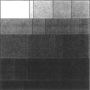
Fig. 1 The slice-and-dice treemap algorithm. Shading indicates order, which is preserved. The left image shows a single level treemap, and the right image shows a hierarchical application of the same algorithm.
A key ingredient of a treemap is the algorithm used to create the nested rectangles that make up the map. (We refer to this set of rectangles as the layout of the treemap.) The slice-and-dice algorithm of the original treemap paper [Shneiderman 1992] uses parallel lines to divide a rectangle representing an item into smaller rectangles representing its children. At each level of hierarchy the orientation of the lines—vertical or horizontal—is switched. Though simple to implement, the slice-and-dice layout often creates layouts that contain many rectangles with a high aspect ratio.1 Such long skinny rectangles can be hard to see, select, compare in size, and label [Bruls et al. 2000; Turo and Johnson 1992]
Several alternative layout algorithms have recently been proposed to address these concerns. The SmartMoney Map of the Market [Smartmoney Marketmap 2002] is an example of the cluster treemap method described in Wattenberg [1999] which uses a simple recursive algorithm that reduces overall aspect ratios. Bruls, Huizing, and van Wijk [2000] introduced the squarified treemap, which uses a different algorithm to achieve the same goal. Figure 2 shows examples of these two layouts.

These methods suffer from several drawbacks. First, changes in the data set can cause dramatic discontinuous changes in the layouts produced by both cluster treemaps and squarified treemaps. (By contrast, the output of the slice and dice algorithm varies continuously with the input data.) These abrupt layout changes are readily apparent to the eye; below we also describe quantitative measurements of the phenomenon. Large layout changes are undesirable for several reasons. If the treemap data is updated on a second-by-second basis (e.g., in a stock portfolio monitor) then frequent layout changes make it hard to track or select an individual item. Rapid layout changes also cause an unattractive flickering that draws attention away from other aspects of the visualization. Moreover, even occasional abrupt changes mean that it is hard to find items on the treemap by memory, decreasing efficacy for long-term users.
A shortcoming of cluster and squarified treemap layouts is that many data sets contain ordering information that is helpful for seeing patterns or for locating particular objects in the map. For instance, the bond data described in Johnson [1994] is naturally ordered by date of maturity and interest rate. In many other cases the given order is alphabetical. The original slice-and-dice layout preserves the given ordering of the data, but cluster treemaps and squarified treemaps do not. Another recent algorithm [Vernier and Nigay 2000] offers some control over the aspect ratios but does not guarantee order. This paper includes a detailed description of a family of algorithms we call “pivot” treemaps (previously called “ordered” treemaps [Shneiderman and Wattenberg 2001]). Using a recursive technique motivated by the QuickSort sorting algorithm, these algorithms offer a trade-off, producing partially ordered layouts that are reasonably stable and have relatively low aspect ratios.
Since treemap algorithms generate visual layouts to be viewed by people, we also must consider the usability of the layouts by people for specific tasks. For someone to look for a particular item using existing algorithms (assuming they are labeled), their eye has to switch between horizontal and vertical scans many times, increasing cognitive load. A layout that has a consistent visual pattern would be easier to search. We propose a measure, which we call readability, that quantifies how easy it is to visually scan a treemap layout, and use it to demonstrate the benefit of ordered layouts. The readability metric counts the number of changes in direction a viewer’s eye must make when scanning the rectangles in order.
We introduce a second ordered treemap algorithm, the “strip” treemap, that is specially designed to produce highly readable displays. A strip treemap layout has a consistently ordered set of rectangles while still maintaining good aspect ratios. Strip treemaps work by creating horizontal rows of rectangles, each with the same height. Implementations of the algorithms as well as an end-user visualization application using these algorithms are available at the University of Maryland’s Human-Computer Interaction Lab web site.2
Another issue with treemap algorithms is what information is displayed in the generated rectangles. In every current usage to date, treemaps are used to visualize a two-dimensional dataset where one dimension is typically mapped to the area of the rectangles (as computed by the treemap algorithm), and the other dimension is mapped to the color of the rectangle. Then, a label is placed in the rectangles that are large enough to accommodate them, and the user can interact with the treemap to get more information about the objects depicted by the rectangles. Surprisingly enough, there are not any published uses of treemaps where other information is placed in the rectangles. We are interested in using treemaps to display large numbers of image thumbnails, clustered by metadata.
There is a good reason why treemaps have not been used in this manner before. This is because while treemaps guarantee that the area of each generated rectangle is proportional to an input number, they do not make any promise about the aspect ratio of the rectangles. Some treemap algorithms (such as squarified treemaps) do generate rectangles with better aspect ratios, but the specific aspect ratio is not guaranteed. While this is fine for general purpose visualizations, it is not appropriate for laying out images because images have fixed aspect ratios, and they do not fit well in rectangles with inappropriate aspect ratios. This paper includes a detailed description and analysis of “quantum” treemaps [Bederson 2001], an approach suitable for laying out images within the generated rectangles.
In this paper, we describe the new ordered and quantum treemap algorithms in detail, along with some experiments that we performed which compare the new treemap algorithms to existing ones using natural metrics for smoothness of updates, overall aspect ratio, and readability. The results suggest that ordered treemaps steer a middle ground, producing layouts with aspect ratios that are far lower than slice-and-dice layouts, though not quite as low as cluster or squarified treemaps; they update significantly more smoothly than clustered or squarified treemaps, though not as smoothly as slice-and-dice layouts; one of the ordered treemaps offers layouts almost as readable as slice-and-dice, which is optimal. Thus ordered treemaps may be a good choice in situations where readability, usability and smooth updating all are important concerns.
Finally, we describe the application of quantum treemaps to a novel photo browser that shows many thumbnails of images, clustered by metadata (where each cluster appears visually within a treemap-generated rectangle). This application, called PhotoMesa, uses a zoomable user interface to enable simple interactions to quickly find the desired photos, while offering the user control over the trade-off between number and resolution of photos presented on the screen.3
2 ORDERED TREEMAP ALGORITHMS
We start by examining ordered treemap algorithms. These are treemap algorithms that create rectangles in a visual order that matches the input to the treemap algorithm. We describe two algorithms. The pivot treemap algorithm [Shneiderman and Wattenberg 2001] creates partially ordered and pretty square layouts while the new strip treemap algorithm creates completely ordered layouts with slightly better aspect ratios.
2.1 The Pivot Treemap Algorithm
The key insight that leads to algorithms for ordered treemaps is that it is possible to create a layout in which items that are next to each other in the input to the algorithm are adjacent in the treemap. The pivot treemap algorithm does not follow the simple linear order of the slice-and-dice layout, but it provides useful cues for locating objects, and turns out to provide constraints on the layout that discourage large discontinuous changes with dynamic data.
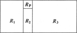
The pivot treemap algorithm follows a simple recursive process, inspired in part by the idea of finding a two-dimensional analogue of the well-known QuickSort algorithm. The inputs are a rectangle R to be subdivided and a list of items that are ordered by an index and have given areas. The first step is to choose a special item, the pivot, which is placed at the side of R. In the second step, the remaining items in the list are assigned to three large rectangles that make up the rest of the display area. Finally, the algorithm is applied recursively to each of these rectangles. The algorithm, as illustrated in Figure 3, can be described as follows. Note that although this assumes the input rectangle is wider than it is tall, the algorithm can be readily modified to accommodate input rectangles that are taller than they are wide, as described in step 3.
Pivot Treemap Algorithm
Input: Rectangle, R, to be subdivided
List of items with area, L1 … Ln
Output: List of rectangles, R1 … Rn
1. If the number of items is <= 4, lay them out in either a pivot, quad, or snake layout as described in the next section, and pick the layout whose average aspect ratio is closest to 1. Stop.
2. Let P, the pivot, be the item with the largest area in the list of items.
3. If the width of R is greater than or equal to the height, divide R into four rectangles, R1, RP, R2, and R3 as shown in Figure 3. (If the height is greater than the width, use the same basic arrangement but flipped along the line y = x.)
4. Put P in the rectangle Rp, whose exact dimensions and position will be determined in Step 5.
5. Divide the items in the list, other than P, into three lists, L1, L2, and L3, to be laid out in R1, R2, and R3. L1, L2 and L3 all may be empty lists. (Note that the contents of these three lists completely determine the placement of the rectangles in Figure 3.) Let L1 consist of all items whose index is less than P in the ordering. Split the remaining items into L2 and L3 such that all items in L2 have an index less than those in L3, and the aspect ratio of RP is as close to 1 as possible.
6. Recursively lay out L1, L2, and L3 (if any are non-empty) in R1, R2, and R3 according to this algorithm by starting at step 1.
2.1.1 Alternate Pivot Selection Strategies.
The algorithm has some minor variations, depending on how the pivot is chosen. The algorithm described in section 2.1 chooses the pivot with the largest area (called pivot-by-size). The motivation for this choice is that the largest item will be the most difficult to place, so it should be done first.
The alternate approaches to pivot selection are pivot-by-middle and pivot-by-split-size. Pivot-by-middle selects the pivot to be the middle item of the list—that is, if the list has n items, the pivot is item number [n/2]. The motivation behind this choice is that it is likely to create a balanced layout. In addition, because the choice of pivot does not depend on the size of the items, the layouts created by this algorithm may not be as sensitive to changes in the data as pivot by size.
Pivot-by-split-size selects the pivot that will split L1 and L3 into approximately equal total areas. The selection works by examining each item and calculating the areas of L1 and L3 as if that item were the pivot. The pivot item that results in the most balanced area between L1 and L3 is chosen. With the sublists containing a similar area, we expect to get a balanced layout, even when the items in one part of the list are a substantially different size than items in the other part of the list. Figure 4 shows examples of the layouts created by these variations.

Fig. 4 Pivot layouts. Shading indicates order, which is roughly preserved. The “P” indicates the first pivot rectangle in each layout.
All pivot selection variations have the property that they create layouts that roughly preserve the ordering of the index of the items, which will fall in a left-to-right and top-to-bottom direction in the layout. The two algorithms are also reasonably efficient: pivot-by-size has performance characteristics similar to QuickSort (order nlog n average case and n2 worst case) while pivot-by-middle has order nlog n performance in the worst case.
Although the variations produce layouts with relatively low aspect ratios (as described in the following sections) they are not optimal in this regard. The stipulations in step 5 of the algorithm avoid some, but not all, degenerate layouts with high aspect ratios, so we experimented with postprocessing strategies designed to improve the layout aspect ratio. For example, we tried adding a last step to the algorithm, in which any rectangle that is divided by a segment parallel to its longest side is changed so that it is divided by a segment parallel to its shortest side. Because this step gave only a small improvement in layout aspect ratio, while dramatically decreasing layout stability, we did not include it in the final algorithm.
2.1.2 End-of-recursion Layout Actions.
Considering a few cases for laying out a small number of items can produce substantially better total results when applied to the layout at the end of the recursion of the pivot treemap algorithm.
The improvement comes from the realization that the layout of rectangles does not necessarily give layouts with the best aspect ratios for all sets of 4 rectangles. In addition, it generates a layout that is somewhat difficult to parse visually because the eye has to move in 3 directions to focus on the 4 rectangles of Figure 3 (horizontally from R1 to RP, vertically from RP to R2, and then horizontally from R2 to R3).
The layout and visual readability can be improved by offering two alternative layouts to the default “pivot” layout. The first alternative produces a “quad” of (2×2) rectangles. The second produces a “snake” layout with all 4 rectangles laid out sequentially—either horizontally or vertically. The snake layout can be equally well applied to 2, 3, or more rectangles. Figure 5 shows the result of laying out a sequence of 4 rectangles using the three stopping conditions.

Fig. 5 Result of applying different layouts to the end of the recutsion with the same set of 4 rectangles.
Since no single layout strategy always gives the best result for all input data, the ordered treemap algorithm computes layouts using all strategies at the stopping condition (pivot, quad, and snake) and picks the best one. In practice, this strategy produces layouts with substantially squarer aspect ratios. We did a test to understand how these layout actions affect aspect ratio. We looked at the average aspect ratios of 100 tests with 100 rectangles each, and random area per rectangle ranging from 10 to 1000. This resulted in an average aspect ratio of 3.9 with the original layout actions, and 2.7 for the new layout actions.
2.2 The Strip Treemap Algorithm
An alternative and simpler strategy gives surprisingly good results. The strip treemap algorithm is a modification of the existing Squarified Treemap algorithm [Bruls et al. 2000]. It works by processing input rectangles in order, and laying them out in horizontal (or vertical) strips of varying thicknesses (Figure 6). It is efficient in that it only looks at rectangles within the strip currently being processed and produces a layout with significantly better readability than the pivot treemap algorithm, with comparable aspect ratios and stability.
As with all treemap algorithms, the inputs are a rectangle R to be subdivided and a list of items that are ordered by an index and have given areas. We describe here, the algorithm for a horizontal layout, but it can easily be altered to produce vertically oriented strips. We maintain a current strip, and then for each rectangle, we check whether adding the rectangle to the current strip will increase or decrease the average aspect ratio of all the rectangles in the strip. If the average aspect ratio decreases (or stays the same), the new rectangle is added. If it increases, a new strip is started with the rectangle.
The layout of any set of rectangles in a strip is completely determined by their order. We calculate the area of the set of rectangles, and from that, and the width of the layout box, we compute the height of the strip. Then, given the height of the strip, we calculate the width of each rectangle so that it has the appropriate area. The algorithm follows. Figure 7 shows the application of the algorithm to a simple input.

Fig. 7 Application of strip treemap application to an input sequence of 5 numbers. At each step (left to right), the algorithm tries adding the new rectangle to the current strip, but creates a new strip if the average aspect ratio of the rectangles in the original strip increases as a result of adding the rectangle. A green checkmark indicates an accepted intermediate layout; a red X indicates one that is suboptimal. The bottom-right layout is the final result.
Strip Treemap Algorithm
Input: Rectangle, R, to be subdivided
List of items with area, L1 … Ln
Output: List of rectangles, R1 … Rn
1. Scale the area of all the items on the input list so that the total area of the input equals that of the layout rectangle.
2. Create a new empty strip, the current strip.
3. Add the next rectangle to the current strip, recomputing the height of the strip based on the area of all the rectangles within the strip as a percentage of the total layout area, and then recomputing the width of each rectangle.
4. If the average aspect ratio of the current strip has increased as a result of adding the rectangle, in step 3, remove the rectangle, pushing it back onto the list of rectangles to process and go to step 2. When the rectangle is removed from a strip, restore that strip to its previous state.
5. If all the rectangles have been processed, stop. Else, go to step 3.
The strip treemap algorithm complexity is understood as follows. For each rectangle, the average aspect ratio of the current strip must be computed, and all the rectangles re-laid out (unless a new strip is started). Each strip is, on average, of length equal to the square root of the total number of rectangles. So, each rectangle on the current strip (sqrt(n)) must be touched for each rectangle in that strip (sqrt(n)) for each of the strips (sqrt(n)), resulting in O(n sqrt(n)) time on average.
As mentioned, this algorithm is similar to the squarified treemap algorithm [Bruls et al. 2000], but the squarified treemap algorithm is different in three ways. First, it sorts the input rectangles by size, which results in better aspect ratios, but (of course) loses the natural order of the rectangles. Second, rather than creating all the strips horizontally, it creates either horizontal or vertical strips in the remaining available space so as to produce the best aspect ratio. Finally, strip treemaps look at the average aspect ratio, while squarified treemaps look at the maximum aspect ratio, of the rectangles in a strip. In this sense, strip treemaps are a simplification of squarified treemaps, resulting in ordered layouts with aspect ratios that are only moderately worse.
The strip treemap algorithm also has some similarity to the space-filling treemap algorithm by Baker et al. [1995]. They designed a strip layout algorithm that does maintain order. But, instead of optimizing aspect ratios, they maintained near-constant strip heights to improve the ability of people to compare the areas of each rectangle. Their algorithm works by deciding in advance the number of strips, and then calculating the strip heights to be of constant height and laying the rectangles out within those strips. However, to avoid splitting rectangles across strips (which could be necessary since the strip heights are calculated independent of their content), they adjust the strip heights to accommodate moving the rectangles to one row or the other.
2.2.1 Lookahead for Strip Treemaps.
The strip treemap algorithm as defined above works well, but frequently has a problem in laying out the last strip. Since the decision to add a rectangle to a strip is made based only on the aspect ratio of the strip being added to, it is possible to be stuck with a few left over rectangles that get placed in a long skinny final strip.
This can be solved in a general way by adding lookahead to the layout. After a strip is constructed with the approach described previously, the next strip is laid out to decide if any rectangles would be better off moved from it to the current strip. The lookahead works as follows: The combined aspect ratio of the rectangles in the current strip, and the aspect ratio of the lookahead strip are compared to what would happen if the rectangles from the lookahead strip were moved to the current strip. If the average aspect ratio is lower when the rectangles are moved to the current strip, they are moved.
Adding lookahead to the strip treemap algorithm eliminates the final skinny strips that can significantly increase the total average aspect ratio. Adding the lookahead function does not change the complexity of the algorithm since the algorithm never processes more than one other strip, which will have, on average, sqrt(n) rectangles. However, the lookahead clearly increases the runtime of any implementation by at least a factor of 2.
2.3 Analysis of Ordered Treemaps
To evaluate the performance of ordered treemap layout algorithms, we compared them to squarified, cluster and slice-and-dice layouts with two experiments, and ran a user study. The first experiment consisted of a sequence of Monte Carlo trials to simulate continuously updating data. Our goal was to measure the average aspect ratio, average layout distance change, and readability produced by each of the algorithms. In the second experiment we measured the average aspect ratio, and readability produced by each of the algorithms for a static set of stock market data. Finally, the user study validated the readability metric by having users search for items in different treemap layouts.
2.3.1 Metrics: Aspect Ratio, Change and Readability.
In order to compare treemap algorithms we define three measures: 1) the average aspect ratio of a treemap layout; 2) a layout distance change function which quantifies how much rectangles move as data is updated; and 3) a readability function which is a measure of how easy it is to visually scan a layout to find a particular item. The ideal would be to have a low average aspect ratio, a low distance change as data is updated, and a high readability, though our experiments suggest that there may be no treemap algorithm that is optimal by all three measures.
We define the average aspect ratio of a treemap layout as the unweighted arithmetic average of the aspect ratios of all leaf-node rectangles, thus the lowest average aspect ratio would be 1.0, which would mean that all the rectangles were perfect squares. This is a natural measure, although certainly not the only possibility. One alternative would be a weighted average that places greater emphasis on larger items, since they contribute more to the overall visual impression. We choose an unweighted average since the chief problems with high aspect ratio rectangles—poor visibility and awkward labeling—are at least as acute for small rectangles as large ones.
The layout distance change function is a metric on the space of treemap layouts that allows us to measure how much two layouts differ, and thus how quickly or slowly the layout produced by a given algorithm changes in response to changes in the data. To define the distance change function, we begin by defining a simple metric on the space of rectangles. Let a rectangle R be defined by a 4-tuple (x,y,w,h) where x and y are the coordinates of the upper left corner and w and h are its width and height. We use the Euclidean metric on this space,—if rectangles R1 and R2 are given by (x1, y1, w1, h1) and (x2, y2, w2, h2) respectively, then the distance between R1 and R2 is given by
We use this metric since it takes into account the visual importance of the shape of a rectangle. A change of 0 would mean that no rectangles moved at all, and the more the rectangles are changed, the higher will be this metric. There are several plausible alternatives to this definition. Two other natural metrics are the Hausdorff metric [Edgar et al. 1995] for compact sets in the plane or a Euclidean metric based on the coordinates of the lower right corner instead of height and width. These metrics differ from the one we chose by a small bounded factor, and hence would not lead to significantly different results.
We then define the layout distance change function as the average distance between each pair of corresponding rectangles in the layouts. We use an unweighted average for the same reasons as we use an unweighted average for aspect ratios.
Finally, the readability metric assigns a numeric value to how easy it is for a person to scan a layout to find a particular item. Scanning relies on an ordered layout since otherwise the entire layout would have to be scanned to find a particular item. We believe that this kind of readability is correlated with the consistency and predictability of a layout. Consistency allows the eye to quickly follow a pattern without having to jump. Predictability allows the eye to jump ahead to the region where the user thinks an item will appear.
We base our readability measure on the number of times that the motion of the reader’s eye changes direction as the treemap layout is scanned in order. To be precise, we consider the sequence of vectors needed to move along the centers of the layout rectangles in order, and count the number of angle changes between successive vectors that are greater than .1 radians (about 6 degrees). To normalize the measure, we divide this count by the total number of rectangles and then subtract from 1. The resulting figure is equal to 1.0 in the most readable case, such as a slice-and-dice layout, and close to zero for a layout in which the order has been shuffled. For a hierarchical layout, we use an average of the readability of the leaf-node layouts, weighted by the number of nodes each contains.
We considered other measures such as counting the average angular difference between rectangles, but decided that once a rectangle sequence changed direction at all, it would force the eye to stop and the amount it had to change direction was not as important as the fact that it changed at all. Since the readability metric given above seems more subjective than the metrics for layout change and aspect ratio, we also performed a user study to validate it.
2.3.2 Monte Carlo trials.
We simulated the performance of the seven layout algorithms under a variety of conditions (slice-and-dice treemaps, pivot treemaps with all three pivot selection strategies, strip treemaps, clustered treemaps, and squarified treemaps). We performed experiments on three types of hierarchies. The first hierarchy (“20×1”) was a collection of 20 items with one level of hierarchy. The second (“100×1”) was a collection of 100 items with one level of hierarchy. The third (“8×3”) was a balanced tree with three levels of hierarchy and eight items at each level for a total of 512 items.
For each experiment we ran 100 trials of 100 steps each. In each experiment we began with data drawn from a log-normal distribution created by exponentiating a normal distribution with mean 0 and variance 1. This distribution is common in naturally occurring positive-valued data [Sheldon 1997]. (Another common distribution, the Zipf distribution, has produced similar results in similar experiments [Shneiderman and Wattenberg 2001].) In each step of a trial the data was modified by multiplying each data item by a random variable ex, where x was drawn from a normal distribution with variance 0.05 and mean 0, thus creating a log-normal random walk. All layouts were created for a square with side 100. The results are shown in Tables I through III.


The results strongly suggest a tradeoff between low aspect ratios and smooth updates. As expected, the slice-and-dice method produces layouts with high aspect ratios, but which change very little as the data changes. The squarified and cluster treemaps are at the opposite end of the spectrum, with low aspect ratios and large changes in layouts. The ordered and strip treemaps fall in the middle of the spectrum.
None produces the lowest aspect ratios, but they are a clear improvement over the slice-and-dice method, with the pivot-by-split-size and strip treemap algorithms producing slightly better aspect ratios. At the same time, they update more smoothly than cluster or squarified treemaps, with the pivot-by-middle algorithm having a slight advantage over the other pivot selection strategies, and the strip treemap doing especially well in the 8×3 case. Aside from the slice-and-dice layouts, strip treemap layouts are by far the most readable in all cases.
2.3.3 Static Stock Market Data.
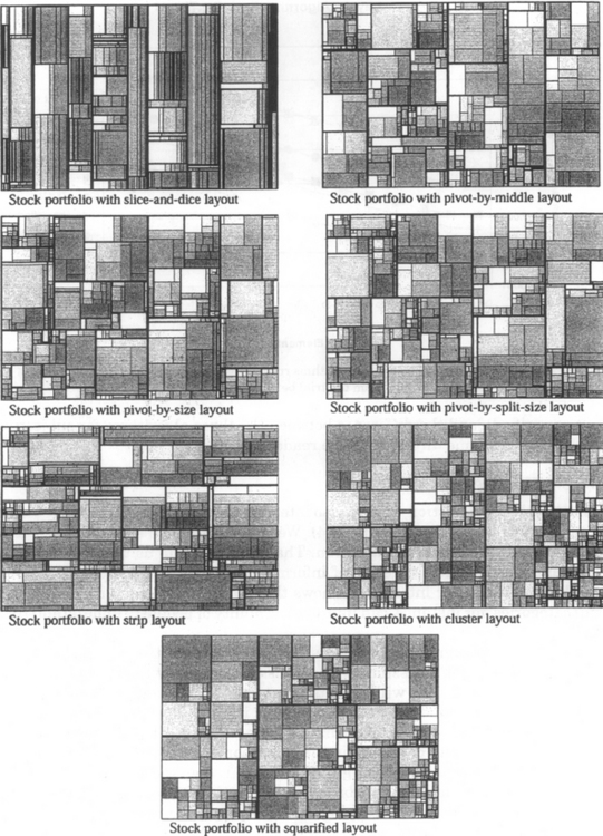
Our second set of experiments consisted of applying each of the seven algorithms to a set of 535 publicly traded companies used in the Smartmoney Map of the Market [Microsoft PowerPoint 2001] with market capitalization as the size attribute. For each algorithm we measured the aspect ratio of the layout it produced. The results are shown in the first column of Table IV, and the layouts produced are shown in Figure 8. (The gray scale indicates ordering within each industry group that is the last level of hierarchy in this data set.) Although aspect ratios are higher than in the statistical trials, partly due to outliers in the data set, the broad pattern of results is similar.

2.3.4 Performance Times.
We compared the actual run-time performance of all of the algorithms discussed in this paper (including quantum strip treemaps from the next section). For this test, we generated flat trees with varying numbers of randomly sized elements (Figure 9). The tests were run on a 700 MHz Pentium III computer running Windows XP. All algorithms were implemented in Java, and were executed with Sun’s JVM, version 1.4. The results match our expectations. The pivot algorithms are the slowest, cluster, squarified, and slice-and-dice are the fastest, and the strip treemaps are in the middle. All algorithms except for the pivot treemaps run fast enough to be practical for even large trees. The strip treemap was able to lay out almost 2,000 rectangles in 0.1 seconds, the cluster and squarified treemaps were able to lay out over 5,000 rectangles in 0.1 seconds, and the slice-and-dice treemap laid out almost 20,000 rectangles in 0.03 seconds.

2.3.5 User Study of Layout Readability.
To validate the readability metric, we performed a user study to see how long it took users to find specific rectangles laid out by different treemap algorithms. We compared the squarified, pivot, and strip treemap algorithms by having participants identify a specific rectangle by clicking on the rectangle with the requested numerical ID. Each algorithm was applied to 100 rectangles with random sizes from a uniform distribution. Each participant did 10 tasks for each of the three algorithms. Each task consisted of a random treemap where each rectangle contained the ID of the rectangle as specified in the input order to the algorithm (Figure 10).
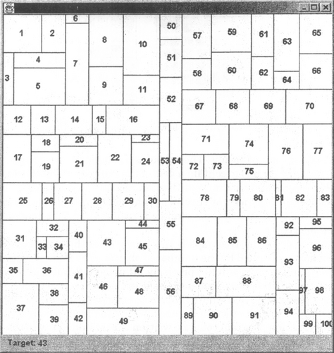
Fig. 10 Screen snapshot from the user study showing what users were presented with when told to click on a specific rectangle. In this case, a pivot treemap was used and the user was told to click on rectangle #43.
The study was run with a completely automated Java application. The participants were first asked some demographic information. Then they were given training tasks followed by the experimental tasks where the participants were instructed to click on the rectangle containing the target number at the bottom of the window. As the participant moved the mouse around, the rectangle under the mouse was highlighted. The study was concluded with each participant rating the three algorithms. So, there was a single independent variable (the treemap algorithm), and two dependent variables (time and subjective preference).
We ran this experiment with 20 participants. The participants were 20% female and 80% male. They were 55% aged 30–39 and 45% aged 20–29. 50% were students. 95% reported using a computer 20 or more hours per week while 5% reported using a computer 10–19 hours per week. The participants reported their primary major or field as being computer science (65%), HCI (15%), informatics (5%), quality assurance (5%), marketing (5%), or unspecified (5%).
We analyzed the results of the experiment by running a single factor ANOVA for the two dependent variables. The measured time (F2,57 = 92.3) p < 0.0001 and subjective preference (F2,57 = 85.6) ρ < 0.0001 each had significant differences, so we performed a post-hoc analysis using Tukey HSD. For the measured time, there was a significant difference between the squarified treemap algorithm and the other two, but not between the pivot and strip treemap algorithms. For subjective preference, there was a significant difference between all three algorithms. Figure 11 shows the numeric results from the experiment.
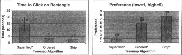
Fig. 11 Results from user study validating readability metric. Error bars show standard deviation, and the algorithms marked with an * are statistically different than the others.
The user study results suggest that the readability metric is predictive of real-world performance on simple search tasks. While the time measurement for the strip and pivot treemap were not significantly different, the trend was in the same direction as the readability metric (strip faster than pivot which is faster than squarified), and the difference between the three algorithms for subjective preference was significant, and in the same direction as the readability metric.
3 QUANTUM TREEMAP ALGORITHMS
As mentioned in the introduction, we are also interested in using treemaps to present clusters of visual information, such as images (see Section 3.4). We would like to be able to lay out images within each rectangle generated by a treemap algorithm. That would enable us to create applications that allow users to see an overview of a large set of information, but grouped in some meaningful way. Some research in human-computer interaction shows that this kind of grouping of search results based on meaningful categories, for instance, can improve the ability of people to understand those search results [Hornof 2001].
Let us look at the problem of applying existing treemap algorithms to laying out fixed size objects, such as images. For now, let us assume without loss of generality that the images are all square (i.e., having an aspect ratio of 1). We will see later that this does not affect layout issues. Given a list of groups of images that we want to lay out, the obvious input to the treemap algorithm is the number of images in each group. The treemap algorithm will generate a list of rectangles, and then we just have to decide how to fit each group of images in the corresponding rectangle.
Since most treemap algorithms give no guarantees about the aspect ratios of the generated rectangles, the images would have to be laid out in arbitrary aspect ratio rectangles which can result in unattractive layouts. Figure 12 shows the result of laying out a simple sequence of images using the pivot treemap and the quantum treemap algorithm we are about to describe. With the quantum treemap algorithm, all images are the same size, and all images are aligned on a single grid across all the groups.

Fig. 12 The result of laying out a sequence of 4 groups of elements (of size 3, 20, 20, 1) using pivot treemap (left) and quantum treemap (right).
3.1 The Quantum Strip Treemap Algorithm (QST)
The quantum treemap algorithm generates rectangles with widths and heights that are integer multiples of a given elemental size. Thus, all the grids of elements will align perfectly with rows and columns of elements running across the entire series of rectangles. It is this basic element size that can not be made any smaller that led to the name of quantum treemaps.
Any treemap algorithm can be quantized, so really quantum treemaps are a family of algorithms that parallel the other treemap algorithms. Quantum treemap’s input and output are similar to those of other treemap algorithms, but instead of taking a list of areas as input, it takes an elemental object dimension, and a list of numbers of objects. The output is a sequence of rectangles where each rectangle is large enough (and possibly larger) to contain a grid of the number of objects requested. The basic idea is to start the regular treemap algorithm and then as rectangles are generated, they are quantized. That is, their dimensions are expanded or shrunk so that each dimension is an integral multiple of the input element size and the total area of the rectangle is no less than that needed to layout a grid of the requested number of objects.
An unusual property of quantum treemaps is that the area of the generated rectangles is typically larger than the object size multiplied by the number of objects to be laid out within that rectangle. The reason for this is that many layouts will not precisely fill up a grid, but will leave some empty cells in the last row. This is obviously true for numbers of objects that are prime (since they have no divisors), but is also true for non-prime numbers where their factors do not generate rectangles that have aspect ratios close to the aspect ratio of the rectangle generated by the treemap algorithm.
While a generic quantization program could be written that would apply to the result of any treemap algorithm, we have instead written custom quantum treemap variations of each ordered treemap algorithm. This is because the custom ones are more efficient (in the amount of wasted space) since they can adapt to the error that is generated by quantized rectangles. We describe here a quantized version of strip treemaps and then summarize the issues that affect quantization of other algorithms.
Quantum Strip Treemap Algorithm (QST)
Input: Rectangle, R, to be subdivided
Elemental object dimensions, D
List of groups with number of objects per group, L1 … Ln
Output: List of rectangles, R1 … Rn
1. Scale R so its area equals the total number of objects in the list L1 … Ln.
2. Create a new empty strip, the current strip.
3. Create a new rectangle to represent the next item on the list, and add it to the current strip. Compute the height of the strip to be the result of rounding up the total number of objects in the groups in the current strip divided by the width of R. Compute the width of each rectangle in the current strip to be the result of rounding up the number of objects in the associated list element divided by the height of the strip.
4. If the average aspect ratio of the current strip has increased as a result of adding the rectangle in step 3, remove the rectangle pushing it back onto the list of rectangles to process, and go to step 2. When the rectangle is removed from a strip, restore that strip to its previous state.
5. If all the rectangles have been processed, continue to step 6. Else, go to step 3.
6. “Justify” the ragged right edge: Compute W, the width of the widest strip. Distribute the extra space of each strip within the rectangles of that strip as follows: For each strip, Si:
Quantizing a treemap algorithm does not change the complexity of the algorithm since it only adds a constant cost to the processing of each rectangle (step 3), and then has a linear clean-up cost (step 6).
3.2 Implementation Details
Quantizing the strip treemap algorithm is somewhat simpler than others because the rectangles in each strip are known to all have the same height. Quantizing other treemap algorithms involves changes similar to the ones we made to the strip treemap, but the changes can sometimes be a bit more subtle since the layouts are not as straightforward as they are for the strip layout. We now look at a few issues that apply to quantization of any treemap algorithm.
3.2.1 Element Aspect Ratio Issues.
Quantum treemaps assume that all the elements to be laid out in the rectangles are the same aspect ratio, and that aspect ratio is an input parameter. It turns out, however, that it is not necessary to modify the internal structure of quantum treemaps to accommodate the element’s aspect ratio. Instead, the dimensions of the starting box can simply be stretched by the inverse of the element aspect ratio. Simply put, laying out wide objects in a wide box is the same as laying out thin objects in a thin box. An example showing images of different aspect ratios is shown in Section 3.4.
3.2.2 Evening Ragged Edges.
For QST, the job of evening the right ragged edge was straightforward since all the rectangles are organized in strips and space could be readily distributed among the rectangles in each strip. For other treemap algorithms, with more complex layouts, handling ragged edges is a bit more subtle. Since the rectangles are not laid out in strips, it is harder to spread extra space among multiple rectangles. It requires working with the area as a whole, and evening the right-most and bottom-most edges.
3.2.3 Growing Horizontally or Vertically.
In the description of QST, we always grew the height of each rectangle, and then changed the width of the rectangle as needed. However, more generally, there is a basic question of which dimension to grow each rectangle. The simple answer is just to grow in the direction that results in a rectangle that most closely matches the aspect ratio of the original rectangle. However, for certain treemap algorithms, it may make more sense to grow in one direction, then another. As we saw for strip treemaps, for example, it makes most sense to have a constant height for each strip, and so we grow the height of each rectangle and then adapt the width.
We have found that the pivot treemap algorithms produce better layouts if they always grow horizontally (or vertically for layout boxes that are oriented vertically). The issue here is somewhat subtle, but is related to the evening of the rectangles. If (looking at Figure 3), for example, rectangles in R3 are made taller, then all of R1 and R2 will have to be made taller as well, to match R3. If instead, the rectangles in R3 are made wider, then only the other rectangles in R3 will need to be made wider, and the rectangles in R1 and R2 can be left alone.
3.3 Analysis of Quantum Treemaps
Quantum treemaps often waste some space, in that it is not always possible to create a rectangular grid that fits the precise number of requested elements. In general, quantum treemaps work better when there are more objects per group. This is because it gives the algorithm more flexibility when computing rectangles. For example, 1000 elements can be arranged in quantized grids of many different sizes such as 30×34 (holds 1020 elements), 31×33 (holds 1023 elements), or 32×32 (holds 1024 elements)—which each use the space quite efficiently, wasting between 20 and 24 elements, or about 2% each. Rectangles containing smaller numbers of elements, however, do not offer as many options, and often use space less efficiently. For example, a rectangle containing 5 elements can be laid out in grids of 1 × 5 or 5 × 1 (holding 5 elements each), or 2×3 or 3×2 (holding 6 elements each). These four options do not give the algorithm as much flexibility as the dozens of grid options afforded by the larger number of elements. In addition, while the 1×5 layouts don’t waste any space, the 2×3 layouts each waste 17% of the space (1 element out of 6).
In order to assess the effectiveness of quantum treemaps, the strip treemap and pivot treemap were compared to the quantized versions of the corresponding algorithm with a series of trials using random input. For each test, the average aspect ratio of all the rectangles was recorded as well as the space utilization, which was recorded as the percentage of space not used to display elements (wasted space). Inefficient use of space is an issue for quantum treemaps because rectangles can be expanded to match nearby rectangles resulting in rectangles larger than necessary to display the objects.
Each algorithm was run 100 times generating 100 rectangles with the number of elements in each rectangle being randomly generated with a uniform distribution. This was done for 5 different ranges of the number of elements per rectangle. The same random numbers were used for each algorithm. Figures 13 and 14 show the results of these tests. Quantum treemaps did better in terms of aspect ratio, and the non-quantized treemaps did better in terms of wasted space.
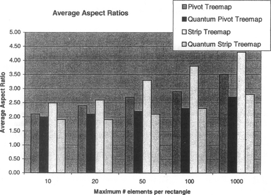
Fig. 13 Average aspect ratio of all rectangles run on both ordered treemap algorithms and their quantized counterparts with 100 rectangles with random numbers of elements per rectangle.

Fig. 14 Average wasted space of all rectangles run on both ordered treemap algorithms and their quantized counterparts with 100 rectangles with random numbers of elements per rectangle.
However, the crucial visual advantage of quantum treemap is that it always produces layouts where elements are the same size and are aligned on a single global grid. So, while understanding the characteristics of quantum treemaps is important, for applications that need them, the importance of their quantum characteristic will typically outweigh the others.
3.4 Application of Quantum Treemaps
We have written an application called PhotoMesa which is an image browser that makes use of quantum strip treemaps to layout groups of images. Figures 15 and 16 show screen snapshots of PhotoMesa which may help to illuminate our interest in this kind of algorithm.


Fig. 16 PhotoMesa using strip treemaps to show the contents of an issue of ACM Interactions magazine. Note the aspect ratio of the images is different than Figure 15.
We designed PhotoMesa to support browsing of personal digital photos targeted for home users. Using metadata from the operating system (directory location, file change dates, and filenames), PhotoMesa groups the photos and lays out the groups using the quantum strip treemap algorithm. PhotoMesa uses a Zoomable User Interface (ZUI) to interact with the photos. Moving the mouse highlights a region of photos, and clicking results in the view smoothly zooming into the highlighted region. Right-clicking zooms out. In this way, users can easily get an overview of 1,000 photos at a time or more, and quickly zoom into photos of interest. Furthermore, this kind of interaction naturally supports serendipitous photo finding. Since so many photos are visible, users are likely to come across other photos of interest while looking for a specific one.
4 CONCLUSION AND FUTURE DIRECTIONS
Treemaps are a popular visualization method for large hierarchical data sets. Although researchers have recently created several algorithms that produce treemap layouts with low aspect ratios, these new algorithms have three drawbacks: they are unstable under updates to the data, they scramble any natural order on the items being mapped, and they are difficult to search for a specific item.
In this paper, we introduced strip treemaps, a new ordered treemap algorithm that generates fairly square aspect ratios. We also explained in detail, pivot treemaps and quantum treemaps, and compared the three algorithms. Through simulation experiments, we evaluated these and three other algorithms (slice-and-dice, cluster, and squarified) to understand the trade-offs between the issues of aspect ratio, order preservation, and stable updates under dynamically changing data. We found that strip treemaps offer the best combination, substantially improving readability while maintaining good aspect ratios and stability, and thus are likely to be preferred for a broad range of applications. However, when stability or aspect ratios are crucial, the slice-and-dice or squarified algorithms, respectively, may be more appropriate.
There are several directions for future research. First, there is room to optimize the ordered treemap algorithms discussed in this paper, especially to improve the overall aspect ratios they produce. It would also be useful to optimize the algorithms used by cluster treemaps and squarified treemaps to improve stability under dynamic updates. Another practical area to explore would be mixing different algorithms to combine their strengths: for instance, using a stable algorithm to lay out high-level nodes and an order-preserving algorithm to lay out leaf nodes might provide a useful combination of global stability and local readability. Or perhaps specific nodes could be anchored to a specific location with other nodes to be laid out around the anchored nodes. More speculatively, since experimental results suggest a tradeoff between aspect ratios and smoothness of layout changes, it would be worthwhile to look for a mathematical theorem that makes this tradeoff precise. It might also be fruitful to explore variants of treemap layouts that can update smoothly by using past layouts as a guide to current ones, or by using tiles that can have nonrectangular shapes [Bederson 2001].
More ambitious goals include accommodation of trees with millions of nodes. Rapid ways of aggregating data and drawing only visible features are necessary, especially to handle continuous updating. This is desirable for monitoring corporate computer networks with thousands of hard drives, stock market trading with millions of transactions, and oil production from thousands of wells and pumps.
Another challenge is to show more than two attribute values for each leaf node, possibly using texture, saturation, sound, or icons. Relationships between nodes might be shown by animation (e.g. blinking), connected lines, textures, or other perceptual methods.
ACKNOWLEDGMENTS
We appreciate the detailed comments of the anonymous reviewers of this paper who offered excellent advice.
REFERENCES
Baker, M. J., Eick, S. G. Space-filling software visualization. J. Vis. Lang. Comput. 1995; 6:119–133.
2 Bederson, B. B., PhotoMesa: A zoomable image browser using quantum treemaps and bubblemaps. UIST 2001, ACM Symposium on User Interface Software and Technology. CHI Letters; 2001;3:71–80.
Bruls, M., Huizing, K., van Wijk, J. J. Squarified treemaps. In: Proceedings of Joint Eurographics and IEEE TCVG Symposium on Visualization (TCVG 2000). IEEE Press; 2000:33–42.
Edgar, G. A., Ewing, J. H., Gehring, F. W. Measure, Topology, and Fractal Geometry. Springer Verlag; 1995.
Fekete, J. -D., Plaisant, C. Interactive Information Visualization to the Million. Tech. Rep. CS-TR-4320, Computer Science Department, University of Maryland, College Park, MD. 2002.
Hornof, A. J. Visual search and mouse pointing in labeled versus unlabeled two-dimensional visual hierarchies. ACM Trans. Computer-Human Interaction. 2001.
Jin, L., Banks, D. C. Tennis Viewer: A browser for competition trees. IEEE Comput. Graph. Appl. 1997; 17(4):63–65.
Johnson, B. Treemaps: Visualizing Hierarchical and Categorical Data. Doctoral dissertation, Computer Science Department, University of Maryland, College Park, MD. 1994.
Jungmeister, W. -A., Turo, D. Adapting Treemaps to Stock Portfolio Visualization. Tech. Rep. CS-TR-2996, Computer Science Department, University of Maryland, College Park, MD. 1992.
Smartmoney Marketmap 2002 http://www. smartmoney. com/marketmap
Sheldon, R. A. A First Course in Probability. Englewood Cliffs, NJ: Prentice Hall; 1997.
Shneiderman, B. Tree visualization with treemaps: A 2-D space-filling approach. ACM Trans. Graph. 1992; 11(1):92–99.
Shneiderman, B., Wattenberg, M. Ordered treemap layouts. In: Proceedings of IEEE Information Visualization (InfoVis 2001). New York: IEEE; 2001:73–78.
Turo, D., Johnson, B. Improving the visualization of hierarchies with treemaps: Design issues and experimentation. In: Proceedings of IEEE Visualization (Visualization 1992). IEEE Press; 1992:124–131.
Vernier, F., Nigay, L. Modifiable treemaps containing variable-shaped units. In: Proceedings of Extended Abstracts of IEEE Information Visualization (InfoVis 2000). New York: IEEE; 2000:28–35.
Wattenberg, M. Visualizing the stock market. In: Proceedings of Extended Abstracts of Human Factors in Computing Systems (CHI 99). ACM Press; 1999:188–189.
1In this paper we define the aspect ratio of a rectangle to mean the maximum of width/height and height/width. Using this definition, the lower the aspect ratio of a rectangle, the more nearly square it is; a square has an aspect ratio of 1, which is the lowest possible value.
2Java open source implementations of all the algorithms we describe here, dynamic demonstrations of these algorithms showing how their trade-offs, and Treemap 3.0—an end-user visualization application using treemaps are all available at http://www.cs.umd.edu/hcil/treemaps
3PhotoMesa is available for download at http://www.cs.umd.edu/hcil/photomesa