
11.3. Detection of Dose-Response Trends
It is commonly agreed that the first step in analyzing dose-response trends and more complex problems related to dose-finding is the assessment of the overall effect of an experimental drug. This step is essentially a screening test to determine whether or not the drug effect exists at all.
Mathematically, the goal of the overall drug effect assessment is to test the null hypothesis of no treatment effect. For example, in the diabetes trial example, clinical researchers were interested in testing whether or not there was any drug-related improvement in the response variable as the infusion rate increased. The corresponding null hypothesis of no treatment effect is given by
where μP is the mean glucose level in the placebo period and μD1, μD2, μD3, μD4 are the mean glucose levels in the four dosing periods. The null hypothesis of no treatment effect is typically tested against the ordered alternative. Under the ordered alternative, the response is assumed to increase monotonically with dose:
In this section we will discuss statistical methods for assessing dose-related trends in the response variable. We will begin with simple contrast tests, discuss powerful isotonic methods (Bartholomew and Williams tests) and introduce a non-parametric approach to testing dose-response trends.
11.3.1. Contrast Tests
The simplest way of testing the null hypothesis of no treatment effect is based on the F test associated with a simple ANOVA model. However, the F test is not especially powerful in a dose-response setting because it does not take advantage of the dose order information. The ANOVA-based approach to examining the overall drug effect can be greatly improved if we select a contrast that mimics the most likely shape of the dose-response curve and carries out a trend test associated with this contrast.
To define contrast tests, consider a general dose-ranging study with m doses of a drug tested versus a placebo. Let θ0 be the true value of the response variable in the placebo group and θ1,...,θm denote the true values of the response variable in the m dose groups. The θ parameters can represent mean values of the response variable when it is continuous or incidence rates when the response variable is binary. Further, let ![]() 0,...,
0,...,![]() m be the sample estimates of the θ parameters in the placebo and dose groups.
m be the sample estimates of the θ parameters in the placebo and dose groups.
A contrast is defined by m + 1 contrast coefficients (one for each treatment group) denoted by
The coefficients are chosen in such a way that they add up to 0, i.e.,
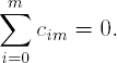
Contrasts are often defined with integer coefficients since the coefficients are standardized when the test statistic is computed.
Once a contrast has been selected, the corresponding t statistic is computed by dividing the weighted sum of the sample estimates ![]() 0,...,
0,...,![]() m by its standard error:
m by its standard error:

In parallel group studies with an equal number of patients in each group (say, n), this statistic follows a t distribution with (m + 1)(n − 1) degrees of freedom.
Popular contrast tests based on linear, modified linear and maximin contrasts are defined below.
11.3.1.1. Linear Contrast
The linear contrast is constructed by assigning integer scores (from 0 to m) to placebo and m ordered doses and then centering them around 0 (Tukey et al, 1985; Rom et al, 1994). In other words, linear contrast coefficients are given by:
Linear contrast coefficients for dose-ranging studies with 2, 3 and 4 dose groups are displayed in Table 11.2.
As was noted above, each contrast roughly mimics the dose-response shape for which it is most powerful. The linear contrast test is sensitive to a variety of positive dose-response shapes, including a linear dose-response relationship. If the test is significant, this does not necessarily imply that the true dose-response relationship is linear.
Secondly, the linear contrast introduced above was originally proposed for dose-response studies with equally spaced doses and equal sample sizes across the treatment groups. However, the same coefficients are frequently used even when these assumptions are violated. When the doses are not equally spaced, the linear contrast essentially becomes an ordinal contrast that ignores the actual dose levels and replaces them with ordinal scores.
11.3.1.2. Maximin and Modified Linear Contrasts
The maximin contrast was derived by Abelson and Tukey (1963) and possesses an interesting optimal property. The contrast maximizes the test's power against the worst-case configuration of the dose effects under the ordered alternative HA:
The maximin contrast is defined as follows:
Along with the optimal maximin contrast, Abelson and Tukey (1963) also proposed a simple modification of the linear contrast that performs almost as well as the maximin contrast. The modified linear contrast (termed the linear-2-4 contrast by Abelson and Tukey) is similar to the linear contrast. The only difference is that the end coefficients are quadrupled and the coefficients next to the end coefficients are doubled. Unlike the maximin coefficients, the modified linear coefficients are easy to compute and remember.
To understand the difference between the linear and maximin tests, note that, unlike the linear tests, the maximin and modified linear tests assign large weights to the treatment means in the placebo and highest dosing groups. As a result, these tests tend to ignore the drug effect in the intermediate dosing groups. Although the maximin and modified linear tests are generally more powerful than the simple linear test, they may perform poorly in trials with non-monotonic dose-response curves.
Maximin and modified linear coefficients for dose-ranging studies with 2, 3 and 4 dose groups are shown in Table 11.2.
| Contrast | Contrast coefficients | ||||
|---|---|---|---|---|---|
| Placebo | Dose 1 | Dose 2 | Dose 3 | Dose 4 | |
| 2 dose groups | |||||
| Linear | −1 | 0 | 1 | ||
| Modified linear | −4 | 0 | 4 | ||
| Maximin | −0.816 | 0 | 0.816 | ||
| 3 dose groups | |||||
| Linear | −3 | −1 | 1 | 3 | |
| Modified linear | −12 | −2 | 2 | 12 | |
| Maximin | −0.866 | −0.134 | 0.134 | 0.866 | |
| 4 dose groups | |||||
| Linear | −2 | −1 | 0 | 1 | 2 |
| Modified linear | −8 | −2 | 0 | 2 | 8 |
| Maximin | −0.894 | −0.201 | 0 | 0.201 | 0.894 |
| Note: The linear and modified linear coefficients have been standardized. | |||||
11.3.2. Contrast Tests in the Diabetes Trial Example
Program 11.1 analyzes changes in fasting serum glucose levels between the placebo and four dosing periods in the diabetes trial example. The raw data (DIABETES data set) used in the program can be found on the book's companion Web site. To account for the cross-over design, the program uses the MIXED procedutre to fit a simple mixed model with a fixed group effect and a random subject effect. The drug effect is assessed using the overall F test as well as the three contrast tests introduced in this section. The contrast coefficients included in the three CONTRAST statements are taken from Table 11.2. Lastly, the program uses the Output Delivery System (ODS) to select relevant sections of the PROC MIXED output.
Example 11-1. F and contrast tests in the diabetes trial example
proc mixed data=diabetes;
    ods select tests3 contrasts;
    class subject rate;
    model glucose=rate/ddfm=satterth;
    repeated/type=un subject=subject;
    contrast "Linear" rate −2 −1 0 1 2;
    contrast "Modified linear" rate −8 −2 0 2 8;
    contrast "Maximin" rate −0.894 −0.201 0 0.201 0.894;
run; |
Example. Output from Program 11.1
Type 3 Tests of Fixed Effects

              Num     Den
Effect         DF      DF    F Value    Pr > F

rate            4    20.2      90.49    <.0001

                     Contrasts

                    Num     Den
Label                DF      DF    F Value    Pr > F

Linear                1    21.3     151.14    <.0001
Modified linear       1    21.6     163.63    <.0001
Maximin 1 21.6 163.56 <.0001 |
Output 11.1 lists the test statistics and associated p-values produced by the overall F test and the linear, modified linear and maximin tests. The test statistics are very large and offer strong evidence against the null hypothesis of no drug effect.
11.3.3. Contrast Tests in the Asthma Trial Example
A similar SAS program can be used to analyze dose-response trends in a parallel group setting, e.g., in the asthma trial introduced in Section 11.1. The only change that needs to be made in Program 11.1 is deleting the REPEATED statement in PROC MIXED. Program 11.2 carries out the overall F test and three contrast tests to analyze mean changes in FEV1 collected in the asthma trial example. The contrast coefficients for this four-arm trial come from Table 11.2. The raw data (ASTHMA data set) used in the program can be found on the book's companion Web site.
Example 11-2. F- and contrast tests in the asthma trial example
proc mixed data=asthma;
    ods select tests3 contrasts;
    class dose;
    model change=dose;
    contrast "Linear" dose −3 −1 1 3;
    contrast "Modified linear" dose −12 −2 2 12;
    contrast "Maximin" dose −0.866 −0.134 0.134 0.866;
run; |
Example. Output from Program 11.2
Type 3 Tests of Fixed Effects

              Num     Den
Effect         DF      DF    F Value    Pr > F

dose            3     104       1.70    0.1707

                     Contrasts

                    Num     Den
Label                DF      DF    F Value    Pr > F

Linear                1     104       1.86    0.1758
Modified linear       1     104       1.86    0.1760
Maximin 1 104 1.85 0.1764 |
Output 11.2 shows the test statistics and p-values produced by the overall F test and the three contrast tests introduced earlier in this section. The four test statistics indicate that the non-monotone (umbrella-shaped) dose-response relationship depicted in Figure 11.2 is actually consistent with the null hypothesis of no drug effect. Note that, in the presence of an umbrella-shaped dose-response curve, the contrast test statistics are comparable in magnitude and are similar to the test statistic of the overall F test.
11.3.4. Isotonic Tests
An alternative approach to testing dose-response trends is based on isotonic []. Unlike contrast tests, isotonic tests rely heavily on the assumption of a monotone dose-response relationship. This assumption is reasonable in most dose-ranging studies because higher doses generally produce stronger treatment effects compared to lower doses.
[] The word isotonic is used in medical literature to describe muscular contractions. In this context, isotonic refers to a monotonically increasing dose-response function.
Two most popular isotonic tests were proposed by Bartholomew (1961) and Williams (1971, 1972). Both of them are based on maximum likelihood estimates of the treatment means under the monotonicity constraint and, as a result, are computationally intensive. Due to the computational complexity of the Bartholomew test, this section will focus on the Williams test for balanced dose-ranging studies with continuous endpoints. It is worth noting the Williams approach can be extended to test for trends in the binary case (Williams, 1988) or in a non-parametric setting (Shirley, 1977).
The Williams trend test is based on a comparison between the highest dose and placebo groups under the monotonicity constraint. To be precise, the Williams test statistic Wm is a two-sample t statistic in which the sample mean in the highest dose group is replaced with the maximum likelihood estimate under the ordered alternative HA:
The Wm statistic is given by

where ![]() 0 is the regular sample mean of the response variable in the placebo group,
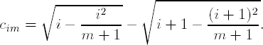
0 is the regular sample mean of the response variable in the placebo group, ![]() m is the maximum likelihood estimate of the average response in the highest dose group under the ordered alternative, s is the pooled sample standard deviation and n is the sample size per group. In the balanced case, the maximum likelihood estimate
m is the maximum likelihood estimate of the average response in the highest dose group under the ordered alternative, s is the pooled sample standard deviation and n is the sample size per group. In the balanced case, the maximum likelihood estimate ![]() m is defined as follows
m is defined as follows
Although the Williams statistic is similar to the two-sample t statistic, it no longer follows a t distribution. To find the critical values of the null distribution of Wm, we need to use a rather complicated algorithm given in Williams (1971). This algorithm is implemented in the PROBMC function. Using this function, we have written a macro for carrying out the Williams test in dose-ranging trials (the %WilliamsTest macro can be found on the book's companion Web site).
The %WilliamsTest macro has three arguments described below:
DATASET is the data set to be analyzed.
GROUP is the name of the group variable in the data set.
VAR is the name of the response variable in the data set.
The macro assumes that the input data set is sorted by the group variable and the first group is the placebo group. Note also that the Williams test was developed for parallel group designs and thus the %WilliamsTest macro will not work with crossover trials.
To illustrate the use of the Williams test, we will apply it to test for a monotonic dose-related relationship in the asthma trial (see Program 11.3).
Example 11-3. Williams test in the asthma trial example
%WilliamsTest(dataset=asthma,group=group,var=change); |
Example. Output from Program 11.3
Williams statistic P-value

1.7339 0.0538 |
Output 11.3 displays the Williams statistic and associated p-value. The p-value is marginally significant (p = 0.0538) and thus the true dose-response relationship in the asthma trial is unlikely to be positive. Also, it is instructive to compare the p-value produced by the Williams test to those produced by popular contrast tests (Output 11.2). The Williams p-value is much smaller than the p-values listed in Output 11.2 which indicates that in this example the Williams test is more sensitive to the dose-response trend than the linear, modified linear and maximin contrast tests.
11.3.5. Jonckheere Test
So far we have discussed dose-response tests for normally or nearly normally distributed endpoints. The assumption of normality may not be met (or may be difficult to justify) in smaller proof-of-concepts trials in which case clinical researchers need to consider a non-parametric test for dose-related trends.
A popular non-parametric trend test for dose-ranging studies was proposed by Jonckheere (1954). A similar test was also described by Terpstra (1952) and, for this reason, the Jonckheere test is sometimes referred to as the Jonckheere-Terpstra test. Another non-parametric trend test was recently proposed by Neuhäuser, Liu, and Hothorn (1998). This test is based on a simple modification of Jonckheere's approach and is more powerful than the original Jonckheere test. However, the Neuhäuser-Liu-Hothorn test is not yet available in SAS.
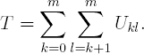
The Jonckheere test is based on counting the number of times a measurement from one treatment group is smaller (or larger) than a measurement from another treatment group and comparing the obtained counts to the counts that would have been observed under the null hypothesis of no drug effect. To define the Jonckheere approach, let Xij be the measurement from the jth patient in the ith treatment group, i = 0,...,m. The magnitude of response in two treatment groups, say, kth and lth groups, can be assessed in a non-parametric fashion using the Mann-Whitney statistic Ukl. This statistic is equal to the number of times Xkj < Xlj' plus one-half the number of times Xkj = Xlj'. The Jonckheere statistic, defined for all pairwise comparisons as a sum of the Mann-Whitney statistic, combines the information across the m + 1 groups.
Once the T statistic has been computed, statistical inferences can be performed using a normal approximation or exact methods. First, one can compute a standardized test statistics which is asymptotically normally distributed and then find a p-value from this normal distribution. Alternatively, a p-value can be computed from the exact distribution of the T statistic.
The Jonckheere test is implemented in the FREQ procedure, which supports both the asymptotic and exact versions of this test. The Jonckheere test (in its asymptotic form) is requested by adding the JT option to the TABLES statement. To illustrate, Program 11.4 carries out the Jonckheere test to examine the dose-response relationship in the asthma trial.
Example 11-4. Jonckheere test in the asthma trial example
proc freq data=asthma;
    tables dose*change/noprint jt;
run; |
Example. Output from Program 11.4
Statistics for Table of dose by change Jonckheere-Terpstra Test Statistic 2450.5000 Z 1.4498 One-sided Pr > Z 0.0736 Two-sided Pr > |Z| 0.1471 Effective Sample Size = 108 Frequency Missing = 4 |
Output 11.4 shows that the standardized Jonckheere statistic for testing the dose-related trend in FEV1 changes is 1.4498. The associated two-sided p-value is fairly large (p = 0.1471) suggesting that the dose-response relationship is not positive.
It is worth noting that PROC FREQ also supports the exact Jonckheere test. To request an exact p-value, we need to use the EXACT statement as shown below
proc freq data=asthma;
    tables dose*change/noprint jt;
    exact jt;
    run;
It is important to remember that exact calculations may take a very long time (even in SAS Release 9.1) and, in some cases, even cause the SAS System to run out of memory.
11.3.6. Comparison of Trend Tests
Several authors, including Shirley (1985), Hothorn (1997) and Phillips (1997, 1998), studied the power of popular trend tests in a dose-ranging setting, including contrast tests (linear and maximin), Williams, Bartholomew and Jonckheere tests.
It is commonly agreed that contrast tests can be attractive in dose-ranging trials because they gain power by pooling information across several dose groups. This power advantage is most pronounced in cases when the shape of the dose-response curve matches the pattern of the contrast coefficients. The contrast tests introduced in this section perform best when the response increases with increasing dose. However, when a non-monotonic (e.g., umbrella-shaped) dose-response curve is encountered, contrast tests become less sensitive and may fail to detect a dose-response relationship. The same is also true for the Jonckheere test.
The isotonic tests (Williams and Bartholomew tests) tend to be more robust than contrast tests and perform well in dose-ranging trials with monotonic and non-monotonic dose-response curves (as shown in Output 11.3). To summarize his conclusions about the performance of various trend tests, Phillips (1998) stated that
specialized tests such as Williams' and Bartholomew's tests which are tailored to the special ordering of dose groups are powerful against a variety of different patterns of results, and therefore, should be used to establish whether or not there is any drug effect.
11.3.7. Sample Size Calculations Based on Linear Contrast Tests
In this subsection, we will briefly discuss a problem that plays a key role in the design of dose-ranging trials—calculation of the trial's size. Consider a clinical trial with a parallel group design in which m doses of an experimental drug are tested against a placebo. The same number of patients, n, will be enrolled in each arm of the trial. The total sample size, n(m + 1), is chosen to ensure that, under a prespecified alternative hypothesis, an appropriate trend test will have 1 − β power to detect a positive dose-response relationship at a significance level α. Here β is the Type II error probability.
Sample size calculations for isotonic tests (Williams and Bartholomew tests) tend to be rather complicated and we will focus on general contrast tests introduced in Section 11.3.1. As before, θ0 will be the true value of the response variable in the placebo group and θ1,...,θm will denote the true values of the response variable in the m dose groups (the response can be a continuous variable or proportion). Suppose that clinical researchers are interested in rejecting the null hypothesis of no drug effect in favor of
where θ0*, θ1*, ...,θm* reflect the assumed magnitude of the response in the placebo and m dose groups. These values play the role of the so-called smallest clinically meaningful difference which is specified when sample size calculations are performed in two-arm clinical trials.
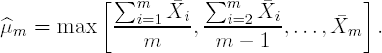
The presence of a positive dose-response relationship will be tested using a general contrast test with the contrast coefficients c0m,c1m,...,cmm. Assume that the standard deviation of ![]() i is σ/√n. It is easy to show that, under HA, the test statistic t, defined in Section 11.3.1, is approximately normally distributed with mean
i is σ/√n. It is easy to show that, under HA, the test statistic t, defined in Section 11.3.1, is approximately normally distributed with mean

and standard deviation 1. Therefore, using simple algebra, the sample size in each arm is given by
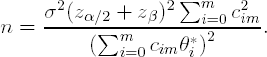
EXAMPLE: Clinical trial in patients with hypercholesterolemia
A clinical trial will be conducted to study the efficacy and safety profiles of three doses of a cholesterol-lowering drug compared to placebo. The primary trial endpoint is the reduction in LDL cholesterol after a 12-week treatment. Clinical researchers hypothesize that the underlying dose-response relationship will be linear, i.e.,
where θ0 is the placebo effect and θ1, θ2 and θ3 represent the drug effect in the low, medium and high dose groups, respectively. The standard deviation of LDL cholesterol changes is expected to vary between 20 and 25 mg/dL. The dose-ranging trial needs to be powered at 90% (β = 0.1) with a two-sided significance level of 0.05 (α/2 = 0.025).
Program 11.5 computes the sample size in this dose-ranging trial using the linear contrast test with c03 = −3, c13 = −1, c23 = 1 and c33 = 3 (see Table 11.2).
Example 11-5. Sample size calculations in the hypercholesterolemia dose-ranging trial
data sample_size;
    * Mean effects in each arm;
    theta0=0; theta1=7; theta2=14; theta3=21;
    * Linear contrast test coefficients;
    c0=-3; c1=-1; c2=1; c3=3;
    alpha=0.025; * One-sided significance level;
    beta=0.1;
    z_alpha=probit(1-alpha);
    z_beta=probit(1-beta);
    do sigma=20 to 25;
        sum1=theta0*c0+theta1*c1+theta2*c2+theta3*c3;
        sum2=c0*c0+c1*c1+c2*c2+c3*c3;
        n=ceil(sum2*(sigma*(z_alpha+z_beta)/sum1)**2);
        output;
    end;
proc print data=sample_size noobs;
    var sigma n;
run; |
Example. Output from Program 11.5
sigma n 20 18 21 19 22 21 23 23 24 25 25 27 |
Output 11.5 lists the patient numbers for the selected values of σ. It is important to remember that these numbers define the size of the analysis population. In order to compute the number of patients that will be enrolled in each treatment group, we need to make assumptions about the dropout rate. With a 10% drop-out rate, the sample size in the first scenario (σ = 20) will be 18/0.9 = 20 patients per arm.