
6.3. The One-Way Layout
The one-way layout is a commonly used experimental design in biological research. A recent Web search of the archival scientific literature (Science Direct) covering the domain of published pharmacological, toxicological and pharmaceutical science research from 2000 to first quarter 2005 produced 3,671 hits pertaining to the application of a one-way layout as the means to address a specific scientific hypothesis. The one-way layout is a powerful means to study basic scientific questions because of its simplicity. Recall that in a one-way layout, experimental units (e.g., subjects) are randomly assigned to two or more treatment groups. The treatment groups could consist of two or more distinct treatments or increasing doses of a single agent (as in the case of later stage drug discovery studies or many standard toxicology investigations). Each unit receives its treatment and a continuous measurement is collected. Formally, consider a study (drug discovery experiment or clinical trial) with ktreatment groups and ni units/subjects in the ith group. Let Xij be the response of the jth experiment unit (j = 1,...,ni) to the ith treatment (i = 1,...,k). The total sample size for the study is N = n1 +...+ nk. Let τi be the effect of the ith treatment group. Then, we can express the relationship between the treatment and response with a simple linear model:
where εij represents the measurement error associated with the jth experimental unit (subject) assigned to the ith group (or treatment). We will assume that the εij's are independent and identically distributed by virtue of the original random assignment of units to treatments.
EXAMPLE: Dopamine Experiment
In an effort to make the discussion more concrete, consider the following simple experiment as an example (Juneau, 2004). Samples of PC12 cells were randomized to one of three groups. The PC12 cells were cultured in one of three media: the first medium was infected with a particular strain of bacteria postulated to be associated with the development of Parkinson's disease. The second group used a medium cultured with a second strain of bacteria. The third group of cells was cultured in a normal uninfected medium. All cells were incubated for 24 hours and harvested to determine the dopamine concentration. Due to some unanticipated circumstances, some samples were lost during processing and the resultant sample sizes were unequal at the end of the study. The dopamine concentration data from this study are included in the DOPAMINE data set provided on the book's companion Web site.
From the formal statement above, Xij would represent the dopamine concentration response of the jth experiment unit (j = 1,...,ni) to the ith treatment (i = 1,2,3), where treatment 1 (control group) sample size is n1 = 14, treatment 2 (Strain I) sample size is n2 = 7, and treatment 3 (Strain II) sample size is n3 = 10.
Typically, researchers will be interested in making decisions about the τi's: "Does evidence exist to declare the response of at least one of the treatment groups to be different from the others?" Mathematically, one could ask: "Is it the case that τ1 = τ2 = ... = τk or does evidence exist to declare at least one τi ≠ τl for i ≠ l?" For the dopamine experiment illustrated previously, this question would translate into "How does the presence of one of the three treatments affect dopamine concentration?" Once again, one could express this question mathematically: "Is it the case that τ1 = τ2 = τ3 or that at least one difference exists amongst all pairs of τ1, τ2, or τ3?"
In some sense, evidence to reject the idea that the treatment effects are all the same is not very informative. Typically, such conclusions do not establish differences in activity amongst several novel agents. Investigators will often be more interested in examining questions with alternatives designed for the comparison of one or more of the treatment effects against a designated group (e.g., a control group) or elucidating where treatment effects exist amongst the k treatments (e.g., pair-wise comparisons). This section will be devoted to the examination of various alternative hypotheses that arise in typical pharmaceutical investigations where the one-way layout is the design of choice.
Section 6.3.1 will address the general alternative hypothesis of unequal treatment effects associated with the Kruskal-Wallis test. Examples will be demonstrated with PROC NPAR1WAY. Section 6.3.2 will deal with nonparametric multiple comparison procedures in the one-way layout when an investigator is interested in comparing all treatment groups against a single designated (control) group or performing all simultaneous pair-wise comparisons of treatment effects. Section 6.3.2 will introduce an original SAS macro code to perform the desired statistical tests.
6.3.1. Testing a General Alternative for k Groups: The Kruskal-Wallis Test
Table 6.4 and Figure 6.3 summarize the dopamine concentration response data collected in the dopamine experiment. Notice the slight asymmetry in the distribution patterns of the control and Strain I-infected samples. The control group has two responses that seem extreme relative to the rest of the measurements.
| Group | Sample size | Mean | Standard deviation | Median | Interquartile range |
|---|---|---|---|---|---|
| Control | 14 | 100.00 | 15.14 | 95.24 | 13.71 |
| Strain I | 7 | 63.12 | 28.65 | 54.29 | 46.38 |
| tSrain II | 10 | 78.04 | 29.81 | 72.98 | 45.12 |
Figure 6-3. Results of the dopamine experiment

A standard approach to comparing these three treatments would be to begin with a classical linear model relating the dopamine response to the treatment:
where for i = 1 (controls), j = 1,...,14; i = 2 (Strain I), j = 1,...,7; i = 3 (Strain II), j = 1,...,10, ηij are independent and identically distributed Gaussian errors (N(0,σ2)), and μ represents the overall population dopamine concentration mean response. This model could then be fit with the GLM procedure. Let's examine a plot of the density of the residuals after fitting the dopamine concentration data with a standard linear model based upon analysis of variance assumptions.
Figure 6-4. Plot of residuals after fitting a traditional analysis of variance-type model in the dopamine experiment
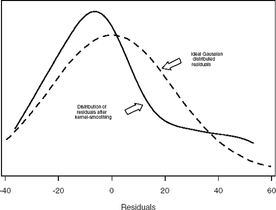
The two curves superimposed in Figure 6.4 allow us to make an interesting conclusion. The dashed curve represents a Gaussian (normal) distribution fitted to the residuals. A solid kernel smooth curve fit to the same residuals suggests that the residuals are asymmetrical (this is also demonstrated by the separation of the means and medians in Table 6.4).
It appears by the evidence presented above that the normality assumption of the ηij's is in question. The typical parametric model and inferences based upon the analysis of variance are thus inappropriate for the evaluation of this experiment. A more appropriate analysis would be based upon the model introduced earlier in this section and the Kruskal-Wallis test (Kruskal and Wallis, 1952).
Consider Model introduced at the beginning of Section 6.3.1 that relates the response of an experimental unit to the effect of the ith treatment τi. The Kruskal-Wallis test is used to test the following null hypothesis against a very general alternative:
- H0 : τ1 = τ2 = ... = τk
versus
- HA : at least one τi ≠ τl for1 ≤ i ≤ k, 1 ≤ l ≤ k, i ≠ l.
In the dopamine study, H0 : τ1 = τ2 = τ3 is tested versus the alternative that states that at least two out of three τ's are different from each other.
The test statistic for the Kruskal-Wallis test is constructed by ranking all N observations from the smallest value to the largest. Tied values are assigned the average rank. The mean rank is then calculated for each group. Denote the mean rank for the ith group by Rī. The Kruskal-Wallis test statistic, K, is then defined by

where T is a correction factor for tied values. If for all N values, ξ groups of size tv (1,2,..., v,..., ξ) exist, the correction factor T is expressed as (Hollander and Wolfe, 1999)

H0 is rejected in favor of HA at level α, if K ≥ cα.
The cutoff value for the test, cα, comes in two varieties. The first is the large sample approximate test, which is based upon a chi-squared cutoff. The degrees of freedom for this test are k − 1, i.e., χk−12(α). The other type of cutoff for this test is the exact version, based upon the permutation distribution of the ranks. PROC NPAR1WAY has had the capability to perform the exact version of the test since SAS Version 6 via the EXACT statement. The formulation of the Kruskal-Wallis statistic and test stated above is not truly an exact α-level test, but only an approximate α-level test. Fortunately, if ties exist in the data, PROC NPAR1WAY will perform the exact α-level test because it determines the permutation distribution of the tied ranks when it determines the p-value for the analysis.
6.3.1.1. Large-Sample Kruskal-Wallis Test
Program 6.7 performs the large-sample Kruskal-Wallis test in the dopamine experiment using PROC NPAR1WAY. The WILCOXON option is used in the procedure to specify Wilcoxon-type scores to perform the Kruskal-Wallis test.
Example 6-7. Large-sample Kruskal-Wallis test in the dopamine experiment
proc npar1way data=dopamine wilcoxon;
    class group;
    var dopamine;
run; |
Example. Output from Program 6.7
Kruskal-Wallis Test

                              Chi-Square         9.0710
                              DF                      2
Pr > Chi-Square 0.0107 |
Output 6.7 shows that the p-value produced by the large-sample Kruskal-Wallis test is 0.0107 and thus we would reject the null hypothesis of equal dopamine response for all three groups in favor of the alternative that at least one difference exists among the three sets of treated samples at α = 0.05.
6.3.1.2. Exact Kruskal-Wallis Test
If we examine the DOPAMINE data set, we notice that several tied responses exist for the dopamine response. Tied values are a reality in many real experiments because of limitations on measurement precision, rounding off of values by scientists, or various other reasons. Let's take advantage of the EXACT statement in PROC NPAR1WAY and see if the results change dramatically (Program 6.8). The program is virtually identical to Program 6.7, with the exception of the insertion of the EXACT statement with a WILCOXON option.
Example 6-8. Exact Kruskal-Wallis test in the dopamine experiment
proc npar1way data=dopamine wilcoxon;
    class group;
    var dopamine;
    exact wilcoxon;
run; |
Example. Output from Program 6.8
Kruskal-Wallis Test

                              Chi-Square                  9.0710
                              DF                               2
                              Asymptotic Pr > Chi-Square  0.0107
Exact Pr >= Chi-Square 0.0074 |
Output 6.8 lists the exact p-value (p = 0.0074), which is also significant at a 0.05 level. It is important to mention that running the exact Kruskal-Wallis test is very resource-intensive. The real time run for this short program and relatively small data set was about three hours long. From the author's perspective, the additional resources required may not justify the implementation of the exact test in this particular setting. This may not always be the case, however. Let's consider another experiment.
EXAMPLE: Hyperplastic Alveolar Nodule (HAN) Study
Samples of four types of cell subsets are prepared for a study of the progression of mouse mammary preneoplastic hyperplastic alveolar nodule (HAN) line C4 to carcinoma. Hoechst fluorescence is measured as a response for each sample. The data from this study are included in the HAN data set given on the book's companion Web site.
Let's assume that the small sample size for this study is enough to warrant the selection of a nonparametric statistical method (see Section 6.1). We also assume that the investigator has a very wide alternative of interest: the investigator is interested in evidence of any difference in response. Does the choice of an exact test or asymptotic test matter? Program 6.9 carries out the large-sample and exact Kruskal-Wallis tests in the HAN study.
Example 6-9. Large-sample and exact Kruskal-Wallis tests in the HAN study
proc npar1way data=han wilcoxon;
    class celltype;
    var fluor;
    exact wilcoxon;
run; |
Example. Output from Program 6.9
Kruskal-Wallis Test

                              Chi-Square                  6.7315
                              DF                               3
                              Asymptotic Pr > Chi-Square  0.0810
Exact Pr >= Chi-Square 0.0383 |
Output 6.9 lists the large-sample and exact p-values produced by the Kruskal-Wallis tests. It appears that if the investigator were interested in using the traditional 0.05 level of statistical significance, he or she might be disappointed with the results of the asymptotic test (p = 0.0810 > 0.05), or elated at the conclusion reached by the exact Kruskal-Wallis analysis (p = 0.0383 < 0.05). The point of this illustration is that small sample sizes can influence the results of a testing procedure and should be considered before an analysis strategy is selected. The next section offers some rules of thumb about group size and about when the asymptotic procedures typically perform reasonably.
6.3.2. Nonparametric Multiple Comparison Procedures for Specific Alternatives
A common objective of many pharmaceutical research investigations with a one-way layout is to compare treatments in a pair-wise fashion. Investigators are typically interested in comparing all treatment responses against one another or in comparing several agents against a designated group (e.g., an inactive control group). Both of these settings involve the simultaneous comparison of several group location parameters (say, means in the parametric case, medians in the nonparametric). It is also often desirable to preserve the family-wise error rate in this inference; i.e., the probability of declaring at least one treatment to be different from another, when in fact, it is not.
If we return to the dopamine experiment first presented in Section 6.3.1, we can see an example of a discovery biology study where investigators might be interested in performing all pair-wise comparisons of treatment groups. The investigators would certainly be interested in comparing the typical response in the Strain I and Strain II infected samples with that of the untreated media samples (control); however, it might be of scientific consequence to know if a difference exists between the two sets of infected samples as well.
6.3.2.1. Dunn's Procedure for All Pair-Wise Comparisons
If an investigator is interested in comparing the location parameters of k experimental groups simultaneously and preserving the family-wise error rate, he or she could use an approach suggested by Dunn (Dunn, 1964) for the linear model introduced previously(6.1), i.e., conclude that τi ≠ τl if
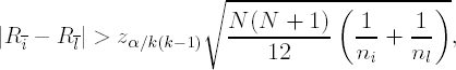
where Rī is the mean of the joint ranks for the ith group, R![]() is the mean of the joint ranks for the lth group, and ni and nl are sample sizes in the two groups, respectively, N is the total sample size, k is the total number of groups (in the dopamine experiment, k = 3) and zα/k(k−1) is the 100α/[k(k−1)]th upper quantile from a standard Gaussian distribution.
is the mean of the joint ranks for the lth group, and ni and nl are sample sizes in the two groups, respectively, N is the total sample size, k is the total number of groups (in the dopamine experiment, k = 3) and zα/k(k−1) is the 100α/[k(k−1)]th upper quantile from a standard Gaussian distribution.
Recall that the joint ranking of a data set is determined by ranking all of the N observations together from smallest to largest.
Dunn's procedure offers the following advantages:
The symmetry assumption, which is often difficult to assess in drug discovery settings with small sample sizes, may be relaxed or ignored.
Equal sample sizes are not required.
Relatively small total sample sizes may be analyzed with this technique, i.e., three groups with five experimental units/group or more than three groups with four units/group (see Lehman, 1975).
6.3.2.2. %DUNN Macro
A simple set of macros can be constructed in SAS to perform Dunn's procedure for all pair-wise comparisons. The author composed a simple SAS macro to perform Dunn's procedure as part of a presentation for the 2004 PharmaSUG meeting in San Diego (Juneau, 2004). The %DUNN macro was designed to imitate PROC NPAR1WAY, with respect to ease of use and input of information, and to produce output quite similar to SAS' very popular procedure, GLM, using the MEANS statement and the CLDIFF option. The macro can be found on the book's companion Web site.
The %DUNN macro consists of a body of code containing one embedded macro (%GROUPS). The embedded macro determines the number of groups present and assigns that value to a macro variable (NGRPS). If a group in the data set does not contain at least one response value (i.e., all values are missing), it will not be included in the analysis. The embedded macro also creates one global macro variable that contains the group labels (GRPVEC) for the levels of the class variable. The main body of the SAS code determines summary statistics (e.g., average ranks, sample sizes, etc.). This information is employed to calculate the pair-wise test statistics. The corresponding cutoff for the test statistic is calculated with the PROBIT function. Results are then printed out using PRINT procedure.
Program 6.10 carries out Dunn's test in the dopamine experiment by invoking the %DUNN macro. The first parameter of the macro is the input SAS data set name (DOPAMINE), the second the classification or grouping variable (GROUP), the third the name of the response variable in the input data set (DOPAMINE), and the fourth macro parameter is the overall family-wise error rate (0.05).
Example 6-10. Large-sample and exact Kruskal-Wallis tests in the HAN study
%dunn(dopamine,group,dopamine,0.05); |
Example. Output from Program 6.10
Large sample approximation multiple comparison procedure
                            designed for unbalanced data
        3 groups: Control StrainI StrainII (respective sample sizes: 14 7 10)
                                    Alpha = 0.05

                                     Difference
                                         in          Cutoff
    Comparison         Group           average         at         Significance
      number        comparisons         ranks      alpha=0.05    difference = **

         1        Control-StrainI      11.8571       10.0759           **
         2        Control-StrainI       7.6429        9.0121
3 StrainI-StrainI 4.2143 10.7266 |
Output 6.10 displays the output of the %DUNN macro. The %DUNN macro produces TITLE statements that state the number of class levels, a list of each of the class levels with non-missing values, and the corresponding group sample sizes. Moreover, the macro generates output that contains the relevant test statistic for each comparison (a function of the average ranks/class level), the corresponding cutoff for the chosen level of family-wise error, and a symbol indicating whether the results of the statistical inference are statistically significant. From this analysis, one would conclude that a statistically significant difference existed between the median dopamine levels in the controls and samples treated with the first strain of bacteria.
6.3.2.3. Dwass-Steel-Critchlow-Fligner Procedure for All Pair-Wise Comparisons
The Dwass-Steel-Critchlow-Fligner (DSCF) procedure is another popular form of simultaneous nonparametric inference in the one-way layout for all pair-wise comparisons (Hollander and Wolfe, 1999). If a pharmaceutical researcher is interested in comparing the location parameters of k experimental groups (τ1,...,τk) simultaneously, and preserving the family-wise error rate, he or she could use an approach suggested by Dwass (Dwass, 1960) and Steel (Steel, 1960) for the linear model previously introduced (6.1).
The procedure begins by calculating the k(k − 1)/2 pairs of Wilcoxon Rank Sum statistics, Wil (Wilcoxon, 1945) for each pair, i and l (1 ≤ i ≤ l ≤ k). The Wilcoxon statistics should include an adjustment for tied values. Conclude that τi ≠ τl if |Dil| > qα,
where

Var(Wil) is the tie-adjusted variance for the Wilcoxon statistic and qα is the 100αth upper quantile from the Studentized Range Distribution (Harter, 1960).
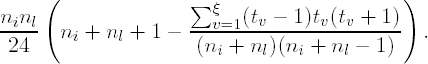
Suppose that for all ni + nl observations in the comparison, ξ tied groups of size tv (1,2,...,v,...,ξ) exist. The variance in the denominator of the statistic is given by (Hollander and Wolfe, 1999)
6.3.2.4. %DSCF Macro
An analysis using the DSCF method may be conducted using a SAS macro called %DSCF created by the author for a 2004 PharmaSUG presentation (Juneau, 2004). The call of the %DSCF macro is as follows:
%dscf(dataset,group,response,alpha);
The first parameter of the macro is the input data set name (DATASET), the second the classification or grouping variable (GROUP), the third the name of the response variable in the input data set (RESPONSE), and the fourth macro parameter is the overall family-wise error rate (ALPHA).
The %DSCF macro consists of a body of code containing one embedded macro (%GROUPS). The embedded macro determines the number of groups present (NGRPS) as in the %DUNN macro. If a group in the input data set does not contain at least one response value, it will be excluded from the analysis. The embedded macro also creates two global macro variables that contain the group labels (GRPVEC) for the levels of the class variable and information about the sample size for each group (NVEC). The main body of the code calculates the necessary summary statistics (e.g., Wilcoxon Rank Sum test statistics) and the number of ties present in each pair-wise comparison. This information is then used to calculate the pair-wise test statistics. The cutoff for the test statistic is calculated with the PROBMC function (using the Studentized Range distribution). As the macro iterates between all pair-wise comparisons it concatenates successive results in a data set called STAT. The final results are then printed out with PROC PRINT.
EXAMPLE: Cardiovascular Discovery Study
Subjects were randomized to one of four treatment groups: three active agents and one vehicle control group. The goal of the experiment was to determine whether the agents could affect triglyceride level (in mg/dl) relative to the vehicle controls and to determine whether evidence existed to declare one agent different from another with respect to triglyceride response. Each subject was treated and, after a fixed post-treatment period, the blood triglyceride level was measured for each subject.
The data gathered in the study are included in the TRIG data set provided on the book's companion Web site. The results of the experiment are displayed in Table 6.5 and Figure 6.5 with box plots and summary statistics. Note the balanced sample sizes. The DSCF multiple comparison method works optimally under settings with equal sample sizes per group.
| Group | Sample size | Mean | Standard deviation | Median | Interquartile range |
|---|---|---|---|---|---|
| Vehicle | 5 | 99.8 | 16.71 | 105.0 | 20.00 |
| Treatment A | 5 | 78.2 | 29.75 | 71.0 | 26.00 |
| Treatment B | 5 | 49.0 | 17.33 | 42.0 | 24.00 |
| Treatment C | 5 | 59.0 | 15.00 | 62.0 | 26.00 |
Figure 6-5. Results of the cardiovascular discovery study

The triglyceride data can be analyzed using the %DSCF macro designed to perform the desired simultaneous pair-wise nonparametric comparisons of all treatments (see Program 6.11).
Example 6-11. Dwass-Steel-Critchlow-Fligner (DSCF) method in the cardiovascular discovery study
%dscf(trig,group,trig,0.05); |
Example. Output from Program 6.11
Large sample approximation multiple comparison procedure
                                  or all treatment pairs
                               based upon pairwise rankings
  4 groups: TreatmentA TreatmentB TreatmentC Vehicle (respective
 sample sizes: 5 5 5 5)
                                       Alpha = 0.05

                                               Test statistic    Cutoff
         Group          Comparison     Test       absolute
         at        Significant
      comparisons         number    statistic       value
      alpha=0.05  difference = **

TreatmentA - TreatmentB      1       −2.21565      2.21565       3.63316
TreatmentA - TreatmentC      2       −1.62481      1.62481       3.63316
TreatmentA - Vehicle         3        1.92023      1.92023       3.63316
TreatmentB - TreatmentC      4        1.92023      1.92023       3.63316
TreatmentB - Vehicle         5        3.69274      3.69274       3.63316         **
TreatmentC - Vehicle 6 3.69274 3.69274 3.63316 ** |
The output of the %DSCF macro in Output 6.11 includes TITLE statements that state the number of class levels, a list of each of the class levels with non-missing values and the corresponding group sample sizes. The macro also lists the relevant test statistic for each comparison (a function of the Wilcoxon statistic), the corresponding cutoff for the chosen level of family-wise error, and a symbol indicating whether the results of the statistical inference are statistically significant. We conclude from Output 6.11 that a statistically significant difference existed between the median triglyceride levels in the controls and samples treated with Treatments B and C. Statistically significant differences did not exist amongst the three active agents (Treatments A, B, and C).
6.3.2.5. Comparison of Dunn and Dwass-Steel-Critchlow-Fligner Methods
Is the DSCF method really necessary, when the multiple comparison procedure suggested by Dunn is a more general case (unequal sample sizes)? The triglyceride data from the cardiovascular discovery study used previously as an example for the application of the DSCF method are analyzed in Program 6.12 with Dunn's method for all pair-wise comparisons.
Example 6-12. Dunn method in the cardiovascular discovery study
%dunn(trig,group,trig,0.05); |
Example. Output from Program 6.12
Large sample approximation multiple comparison procedure
                            designed for unbalanced data
4 groups: TreatmentA TreatmentB TreatmentC Vehicle (respective sample sizes: 5 5 5 5)
                                    Alpha = 0.05

                                        Difference
                                            in          Cutoff
 Comparison            Group              average         at         Significance
   number           comparisons            ranks      alpha=0.05    difference = **

      1        TreatmentA-TreatmentB        6.6         9.87145
      2        TreatmentA-TreatmentC        3.6         9.87145
      3        TreatmentA-Vehicle           5.0         9.87145
      4        TreatmentB-TreatmentC        3.0         9.87145
      5        TreatmentB-Vehicle          11.6         9.87145           **
6 TreatmentC-Vehicle 8.6 9.87145 |
It is instructive to compare Output 6.11 (DSCF method) and Output 6.12 (Dunn method). Recall that in Output 6.11, Treatment C was also declared to be statistically significantly different from the vehicle control group for the median triglyceride response. A comparison of the properties of these two methods may shed some light on the reason for the differing inferential conclusions. First, the Dunn method uses a Bonferroni-like correction to the family-wise error rate (Miller, 1981) and might be a bit too conservative. Second, the Dunn method employs joint ranking, and thus the comparison of two groups is highly influenced by the behavior of other groups in the experiment as the data are initially ranked over the entire experiment (Hollander and Wolfe, 1999). The balanced sample sizes for all groups also suggest that the DSCF method might be the most appropriate technique to employ for all pair-wise nonparametric comparisons.
6.3.2.6. Simultaneous Nonparametric Inference in the One-Way Layout for All Group Comparisons with a Designated Control Group
It is often the case that investigators are interested in comparing the location parameters of treatments against the location parameter of a designated group. This designated group could be a control group consisting of the response of subjects or units completely untreated by any form of active agent. These are often referred to as untreated control subjects or units. More commonly, a group of experimental units or subjects treated with the vehicle, or medium for delivery of the compound, is the designated group of interest. Such subjects or units are referred to as forming the vehicle control group. A third type of control group is a set of subjects or units treated with an agent known to provoke a response that is the same as one desired by proponents of one of the compounds under examination. Such a collection of subjects or units is called a positive control group.
Other forms of designated control groups exist. The point, however, is that if pharmaceutical researchers are interested in comparing the location parameters of several experimental groups (τ1,...,τk) to a designated group (τc), simultaneously and preserving the family-wise error rate, they can use one of two approaches originallysuggested by Dunn (Dunn, 1964) or Miller (Miller, 1966) for the linear model (6.1). These approaches are described below.
6.3.2.7. Dunn's Method for All Group Comparisons to a Designated Control Group (Unequal Sample Sizes)
Using the notation first introduced in the beginning of Section 6.3, suppose that ni ≠ nj for at least one (i,j) pair (1 ≤ i < j ≤ k) of treatments. We could conclude that τi ≠ τc if
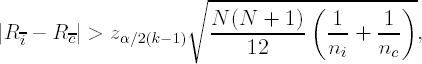
where Rī is the mean of the joint ranks for the group i, R![]() is the mean of the joint ranks for the control group c, and ni and nc are sample sizes for group i and the control group, c, respectively, N is the total sample size, k − 1 is the total number of comparisons desired and zα/2(k−1) is the 100α/[2(k − 1)]th upper quantile from a standard Gaussian distribution.
is the mean of the joint ranks for the control group c, and ni and nc are sample sizes for group i and the control group, c, respectively, N is the total sample size, k − 1 is the total number of comparisons desired and zα/2(k−1) is the 100α/[2(k − 1)]th upper quantile from a standard Gaussian distribution.
6.3.2.8. Miller's Method for all Group Comparisons to a Designated Control Group (Equal Sample Sizes)
Using the notation introduced above, assume that ni = nj for all (i,j) pairs (1 ≤ i < j ≤ k) of treatments. Then τi is declared different from τc if
where Rī, R![]() , ni, nc, N, K are defined as above and |Mα,k−1,∞| is the αth quantile from the Studentized Maximum Modulus distribution (Pillai and Ramachandran, 1954).
, ni, nc, N, K are defined as above and |Mα,k−1,∞| is the αth quantile from the Studentized Maximum Modulus distribution (Pillai and Ramachandran, 1954).
6.3.2.9. %NPARMCC Macro
All nonparametric pair-wise comparisons to a designated control group in a one-way layout can be performed with the %NPARMCC macro that can be found on the book's companion Web site. The macro consists of a body of code containing one embedded macro (%GROUPS). The embedded macro determines the number of groups present (NGRPS) as in the %DUNN and %DSCF macros. If a group in the SAS data set does not contain at least one response value, it will be excluded from the analysis. The embedded macro also creates one global macro variable that contains the group labels (GRPVEC) for the levels of the class variable. The main body of the macro determines the necessary summary statistics (e.g., average ranks, sample sizes, etc.). This information is then employed to calculate the pair-wise test statistics. The cutoff for the test statistic is calculated with the PROBIT function for Dunn's method and the PROBMC function (with the Studentized Maximum Modulus distribution) for Miller's method. The results are then printed out with PROC PRINT.
EXAMPLE: Thrombosis Experiment
An experiment was designed to study the effect of increasing the dose of a novel agent on activated clotting time (ACT). Subjects were randomized to one of four groups: a vehicle control group, a low dose group, a medium dose group, and a high dose group. About 200 minutes after receiving treatment, the ACT for each subject was measured (in seconds). The data from this experiment are contained in the THROMB data set (available on the book's companion Web site) and its results are shown in Table 6.6 and Figure 6.6 (as before, with box plots and summary statistics).
| Group | Sample size | Mean | Standard deviation | Median | Interquartile range |
|---|---|---|---|---|---|
| Control | 5 | 64.2 | 8.11 | 63.0 | 6.00 |
| Low dose | 5 | 98.4 | 17.47 | 106.0 | 14.00 |
| Middle dose | 5 | 91.8 | 14.06 | 98.0 | 16.00 |
| High dose | 5 | 156.4 | 9.40 | 153.0 | 2.00 |
Figure 6-6. Results of the thrombosis experiment
The thrombosis experiment data can be analyzed using the %NPARMCC macro designed to perform the desired simultaneous pair-wise nonparametric comparisons of all groups against a designated control group. Program 6.13 applies the %NPARMCC macro to the THROMB data.
Example 6-13. Dunn's and Miller's methods in the thrombosis experiment
%nparmcc(thromb,group,Control,act,0.05); |
Example. Output from Program 6.13
Large sample approximation multiple comparison procedure
           for all treatment compared against a control (control group = Control)
       4 groups: Control HighDose LowDose MedDose (respective sample sizes: 5 5 5 5)
                                      Alpha = 0.05

                            Difference    Dunn      Miller
                                in       cutoff     cutoff
    Significant   Significant
      Group      Comparison   average      at         at      difference    difference
   comparisons     number      ranks    alpha=0.05 alpha=0.05
 Dunn's = *D*  Miller's = *D*

HighDose-Control      1         14.6     8.95745    8.93410       *D*           *M*
LowDose-Control       2          7.6     8.95745    8.93410
MedDose-Control 3 6.2 8.95745 8.93410 |
The output of the %NPARMCC macro displayed in Output 6.13 includes a list of the class levels with non-missing values, corresponding group sample sizes, and relevant test statistic for each comparison (the difference in the mean ranks), the corresponding cutoff for the chosen level of family-wise error, and a symbol indicating whether the results of the statistical inference are statistically significant by Dunn's method (*D*) and Miller's method (*M*). We conclude from Output 6.13 that a statistically significant difference existed between the median activated clotting time in the controls and samples treated with high dose of the new agent. As the experiment consisted of balanced sample sizes, the conclusion presented by the Miller approach would be considered the appropriate one to report.
6.3.2.10. Comparison of Dunn's and Miller's Methods for All Pair-Wise Comparisons Versus a Designated Control Group
It is interesting to compare the behavior of Dunn's and Miller's respective methods using a data set that is not balanced with respect to sample size. Suppose that we conducted a similar thrombosis experiment as described previously a second time, yet this time with unequal sample sizes. The experimental results are slightly different (the control and low dose groups have different sample sizes than in the original thrombosis experiment). The results are summarized in Table 6.7 and Figure 6.7. The data from this study are included in the THROMB2 data set available on the book's companion Web site.
| Group | Sample size | Mean | Standard deviation | Median | Interquartile range |
|---|---|---|---|---|---|
| Control | 9 | 62.2 | 11.10 | 63.0 | 6.00 |
| Low dose | 8 | 100.0 | 20.87 | 98.5 | 26.00 |
| Middle dose | 5 | 96.4 | 18.37 | 106.0 | 24.00 |
| High dose | 5 | 144.4 | 31.63 | 153.0 | 2.00 |
Figure 6-7. Results of the thrombosis experiment with unequal sample sizes
The data from the thrombosis experiment with unequal sample sizes were once again analyzed using the %NPARMCC macro (Program 6.14).
Example 6-14. Dunn's and Miller's methods in the thrombosis experiment with unequal sample sizes
%nparmcc(thromb2,group,Control,act,0.05); |
Example. Output from Program 6.14
Large sample approximation multiple comparison procedure
            for all treatment compared against a control (control group = Control)
        4 groups: Control HighDose LowDose MedDose (respective sample sizes: 9 5 8 5)
                                         Alpha = 0.05

                            Difference   Dunn       Miller
                               in       cutoff      cutoff
     Significant   Significant
Group           Comparison   average      at          at
       difference    difference
comparisons       number      ranks    alpha=0.05  alpha=0.05
  Dunn's = *D*  Miller's = *D*

HighDose-Control    1       17.4667     9.42126     10.5710        *D*          *M*
LowDose-Control     2       10.2917     8.20747      9.2091        *D*          *M*
MedDose-Control 3 10.1667 9.42126 10.5710 *D* |
Output 6.14 displays the cutoffs computed by the %NPARMCC macro in the modified thrombosis experiment data set. The results of the analysis are quite interesting. Note that Miller's method does not declare the median response for the medium dose group to be statistically significantly different from the control group, while Dunn's method does declare this result to be statistically significant. The difference in the inferential conclusions can be attributed to the fact that Dunn's method was derived to handle the unequal sample size setting, whereas the Miller method, using the Studentized Maximum Modulus cutoff, works optimally under conditions of equal sample size (Hochberg and Tamhane, 1987).
6.3.2.11. Summarization of the Nonparametric Multiple Comparison Methods
Table 6.8 summarizes the nonparametric methods presented in this section and provides advice on the method to use given the study design of a particular investigation.
| Desired comparison | Study design feature | Nonparametric method | SAS macro to perform analysis |
|---|---|---|---|
| All pair-wise comparison | Equal group sample sizes | Dwass-Steel-Critchlow-Fligner method | %DSCF |
| Unequal group sample sizes | Dunn's method | %Dunn | |
| Comparisons with a designated control group | Equal group sample sizes | Miller's method | %NPARMCC |
| Unequal group sample sizes | Dunn's method | %NPARMCC |
6.3.3. Summary
The one-way layout is commonly used in scientific investigations in the pharmaceutical industry. For asymmetrical response data, nonparametric statistical methods offer data analysis methods for a general alternatives of at least one change in location (Kruskal-Wallis test) or more specific, such as all pair-wise comparisons of treatment group locations (Dunn and Dwass-Steel-Critchlow-Fligner methods) or comparisons with a designated control group (Dunn and Miller methods). All techniques can be useful in settings where a small number of responses in a group skew responses or adversely affect the mean response. As was the case for the two-sample setting, it is important to study data properties (i.e., balanced vs. unbalanced sample sizes) before selecting a statistical method.