
Contents
Summarize Columns
The Tables > Summary command calculates various summary statistics, including the mean and median, standard deviation, minimum and maximum value, and so on.
In a summary table:
• A single row exists for each level of a grouping variable that you specify. If no grouping variable is specified, a single row exists for the full data table.
• When there are several grouping variables, the table contains rows for each combination of levels of all the grouping variables.
• In addition to one column for each grouping variable, the table contains frequency counts in a column named N Rows with counts for each grouping level.
• The summary table can be linked to its source table. When you select rows in the summary table, the corresponding rows are highlighted in its source table.
• If the source table’s column(s) contain value labels, the value labels are displayed in the new table.
• A summary table is not saved when you close it unless you select File > Save As to give it a name and location.
Create a Summary Table
To create a summary table:
1. Open a data table.
2. Select Tables > Summary. The window in Figure 8.2 appears.
3. Highlight the columns that you want to summarize.
Note: For details about the options in the red triangle menu, see the Basic Analysis and Graphing book.
Figure 8.2 The Summary Window

4. Add summary statistics, groups, subgroups, and select any options needed:
5. Name the summary table by typing a name in the box beside Output table name.
6. Click OK.
Add Summary Statistics
You can add columns that display summary statistics (such as mean, standard deviation, median, and so on) for any numeric column in the source table.
1. In the Summary window, highlight the column that you want to use in calculating the statistics.
2. Click the Statistics button.
3. Select one of the standard univariate descriptive statistics from the Statistics drop-down menu. The statistics are described in Explanation of Statistics.
Use One or More Grouping Columns
If you want the statistics summarized by group, highlight the column(s) that you want to be your grouping variables and click Group to move the variable into the grouping variables list. See Example of Creating a Summary Table, for an example. If you add only grouping variables, the summary table shows a count for each group.
To change the order of the grouping variables:
To change the order of the grouping variables (ascending or descending order), select a variable in the grouping variable list and click the ascending or descending button ( ). The icon beside the variable changes to indicate the sorting order.
You can also change the order of the grouping variables using the Value Ordering column property. See Value Ordering in Set Column Properties.
To include marginal statistics:
To add marginal statistics (for the grouping variables) to the output columns, click the box beside Include marginal statistics. In addition to adding marginal statistics for each grouping variable, JMP adds rows at the end of the table that summarize each level of the first grouping variable. For example, proceed as follows:
1. Open the Companies.jmp sample data table.
2. Select Tables > Summary.
3. Select Profits ($M) and click Statistics.
4. Select Mean.
5. Select Type and Size Co and click Group.
6. Select Include marginal statistics.
7. Click OK (or Create). See Figure 8.3 at left.
Figure 8.3 Summary Table with and without Marginal Statistics

Compare the summary table with marginal statistics (at left) to the summary table without marginal statistics (at right). You can see that the marginal statistics are added, and a row showing that there are 32 total Computer and Pharmaceutical companies.
Use Quantile Statistics
To add specific quantile statistics, follow these steps:
1. In the box under For quantile statistics, enter value (%) type the desired quantile value (%) for the first quantile (for example, 25).
2. Select the applicable column and click Statistics.
3. Select Quantiles.
4. (Optional) Repeat this process for any additional quantiles.
Change the Format of the Statistics Column Name
To change the format of the statistics column name in the summary table, select from one of the formats in the statistics column name format menu. Table 8.1 illustrates the available options. Assume that you are creating a summary table of the mean profits for a company. Your original column name is Profits ($M).
|
Option
|
Example
|
|
stat (column)
|
Mean (Profits ($M))
|
|
column
|
Profits ($M)
|
|
stat of column
|
Mean of Profits ($M)
|
|
column stat
|
Profits ($M) Mean
|
Link to the Original Data Table
You can select whether to link the summary table to the original data table. By default, the Link to original data table option is selected. If you want to edit the data in the summary table, deselect the Link to original data table option. When the summary table is linked to the original data table, you cannot edit the data in the summary table, since that would modify and compromise the original data.
Within linked tables, if you drag and drop columns from the summary table into the column heading of a new column in the original data table, the values are expanded as if they were matched by grouping columns.
Keep the Summary Window Open
If you select the Keep dialog open option, the Summary window remains open after you click Create. Notice that once you select this option, the OK button is replaced by a Create button.
Create a Two-Way Table of Summary Statistics by Adding a Subgroup Variable
1. Highlight the column(s) that you want to be the nested variable(s). These are your “subgroup variable(s).”
2. Click Subgroup to move the variable(s) into the subgroup list.
3. Highlight the column for which you want statistics summarized by subgroup.
4. In the Statistics list, select the specific statistic that you want.
5. Click OK.
For details about the types of statistics, see Explanation of Statistics.
Add a Statistics Column to an Existing Summary Table
After you have created a summary table, you can add columns of descriptive summary statistics for any numeric column in the source table. To do so, from an existing summary table, click on the upper red triangle in the data grid and select Add Statistics Column.
Example of Adding a Statistics Column to an Existing Table
Suppose that you have already created a summary table, and you want to add more statistics to the existing summary table.
1. Open the Companies.jmp sample data table.
2. Select Tables > Summary.
3. Select Type and Size Co and click Group.
4. Click OK (or Create).
5. From the red triangle menu in the upper left corner of the data table grid, select Add Statistics Column.
Figure 8.4 Creating a Summary Statistics Column from Within a Data Table

A modified version of the Summary window appears.
6. Select the column that you want, click Statistics, and select the specific statistic that you want. For this example, select profit/emp and click Statistics, and then select Mean.
7. Click OK.
Figure 8.5 Example of a Summary Table with a Summary Statistics Column

The Mean(profit/emp) column is added to the existing summary table.
Explanation of Statistics
You can add columns of descriptive summary statistics for any numeric column in the source table by clicking the Statistics button (Figure 8.6) and making a selection from the menu.
Figure 8.6 Adding Summary Statistics

The Statistics menu gives these summary statistics for numeric columns:
• N Is the number of nonmissing values.
• Mean Is the arithmetic mean of a column’s values. It is the sum of nonmissing values (and if defined, multiplied by the weight variable) divided by the Sum Wgt.
• Std Dev Is the sample standard deviation, computed for the nonmissing values. It is the square root of the sample variance.
• Min Is the smallest nonmissing value in a column.
• Max Is the largest nonmissing value in a column.
• Range Is the difference between Max and Min.
• % of Total Is the percent of the total count for each group. Or, if you have so specified, the percent of nonmissing values of the column to the total count for each group.
• N Missing Is the number of missing values.
• Sum Is the sum of all values in a column.
• Sum Wgt Is the sum of all weight values in a column. (See Assign Column Properties in Set Column Properties.) Or, if no column is assigned the weight role, Sum Wgt is the total number of nonmissing values.
• Variance Is the sample variance, computed for the nonmissing values. It is the sum of squared deviations from the mean, divided by the number of nonmissing values minus one.
• Std Err Is the standard error of the mean. It is the standard deviation divided by the square root of N. If a column is assigned the role of weight, then the denominator is the square root of the sum of the weights.
• CV (Coefficient of Variation) Is the measure of dispersion, which is the standard deviation divided by the mean multiplied by one hundred.
• Median Is the 50th percentile, which is the value where half the data are below and half are above or equal to the 50th quantile (median).
• Quantiles Gives the value at which the specific percentage of the argument is less than or equal to. For example, 75% of the data is less than the 75th quantile. The summary window has an edit box for entering the quantile percentage that you want.
Example of Creating a Summary Table
Suppose a researcher is working with Companies.jmp, which groups companies by Type and Size. Follow along with this next example by opening Companies.jmp from the Sample Data folder that was installed when you installed JMP.
Suppose the researcher wants to:
• Create a table that shows the average profit per employee for small, medium, and big computer and pharmaceutical companies. In other words, create a table that contains a row for each size company and a column for the mean profit per employee of each type of company.
• Create it so the cells hold the mean for the subgroup (defined by the intersection of the row and column).
1. Open the Companies.jmp sample data table.
2. Select Tables > Summary.
3. Select Size Co and click Group.
The researcher selects Size Co as the grouping variable because he wants the values in that column to become rows in the new table.
4. Select profit/emp and click Statistics.
5. Select Mean.
6. Select Type and click Subgroup.
This tells JMP to create a column for the average profit per employee (Mean(profit/emp)) for each level (computer, pharmaceutical) of subgroup variable (type).
Figure 8.7 shows the completed Summary window and the resulting summary table.
Figure 8.7 Summary Statistics for a Subgroup

Tabulate Data
Use the Tables > Tabulate command for constructing tables of descriptive statistics. The tables are built from grouping columns, analysis columns, and statistics keywords. Through its interactive interface for defining and modifying tables, the Tabulate command provides a powerful and flexible way to present summary data in tabular form, as shown in Figure 8.8.
Figure 8.8 Examples of Tables

Create a Table in Tabulate
A report in Tabulate consists of one or more column tables concatenated side by side, and one or more row tables concatenated top to bottom. A report might have only a column table or a row table.
Creating a table using the interactive table is an iterative process:
1. Click and drag the items (column name from the column list or statistics from the keywords list) from the appropriate list. Refer to the description of the elements in the interactive table in Elements of a Table in Tabulate.
Note: For details about the options in the red triangle menu, see the Basic Analysis and Graphing book.
2. Drop the items onto the dimension (row table or column table) where you want to place the items’ labels. (See Click and Drag Items, and Elements of a Table in Tabulate, for details.)
3. After creating a table, add to it by repeating the above process. The table updates to reflect the latest addition. If there are already column headings or row labels, you decide where the addition goes relative to the existing items.
Elements of a Table in Tabulate
In Tabulate, a table is defined by its column headings and row labels. They are referred to as the column table and the row table. For a description of column tables and row tables, see Column Tables and Row Tables.
Grouping Columns
Grouping columns are columns that you want to use to classify your data into categories of information. They can have character, integer, or even decimal values, but the number of unique values should be limited.
Note the following:
• If there is more than one grouping column, Tabulate constructs distinct categories from the hierarchical nesting of the values of the columns. For example, from the grouping columns Sex with values F and M, and the grouping column Marital Status with values Married and Single, Tabulate constructs four distinct categories: F and Married, F and Single, M and Married, M and Single.
• You can specify grouping columns for column tables as well as row tables. Together they generate the categories that define each table cell.
• Tabulate does not include observations with a missing value for one or more grouping columns by default. You can include them by checking the Include missing for grouping columns option.
• To specify codes or values that should be treated as missing, use the Missing Value Codes column property. You can include these by checking the Include missing for grouping columns option. See Missing Value Codes in Set Column Properties.
Analysis Columns
Analysis columns are any numeric columns for which you want to compute statistics. They are usually continuous columns. Tabulate computes statistics on the analysis columns for each category formed from the grouping columns.
Note that all the analysis columns have to reside in the same dimension, either in the row table or in the column table.
Statistics
Tabulate supports a list of standard statistics. The list is displayed in the control panel. You can drag any keyword from that list to the table, just like you do with the columns. Note the following:
• The statistics associated with each cell are calculated on values of the analysis columns from all observations in that category, as defined by the grouping columns.
• All of the requested statistics have to reside in the same dimension, either in the row table or in the column table.
• If you drag a continuous column into a data area, it is treated as an analysis column.
Some of the keywords used in Tabulate are defined below. A comprehensive description is listed in Explanation of Statistics.
• N provides the number of nonmissing values in the column. This is the default statistic when there is no analysis column.
• Sum is the sum of all values in the column. This is the default statistic for analysis columns when there are no other statistics for the table.
• Quantiles gives the value at which the specific percentage of the argument is less than or equal to. For example, 75% of the data is less than the 75th quantile. You can request different quantiles by clicking and dragging the Quantiles keyword into the table, and then entering the quantile into the box that appears.
• % of Total computes the percentage of total of the whole population. The denominator used in the computation is the total of all the included observations, and the numerator is the total for the category. If there is no analysis column, the % of Total is the percentage of total of counts. If there is an analysis column, the % of Total is the percentage of the total of the sum of the analysis column. Thus, the denominator is the sum of the analysis column over all the included observations, and the numerator is the sum of the analysis column for that category. You can request different percentages by dragging the keyword into the table.
– Dropping one or more grouping columns from the table to the % of Total heading changes the denominator definition. For this, Tabulate uses the sum of these grouping columns for the denominator.
– To get the percentage of the column total, drag all the grouping columns on the row table and drop them onto the % of Total heading (same as Column %). Similarly, to get the percentage of the row total, drag all grouping columns on the column table and drop them onto the % of Total heading (same as Row %).
• Column % is the percent of each cell count to its column total if there is no analysis column. If there is an analysis column, the Column % is the percent of the column total of the sum of the analysis column.
• Row % is the percent of each cell count to its row total if there is no analysis column. If there is an analysis column, the Row % is the percent of the row total of the sum of the analysis column.
• All is a special keyword for grouping columns. It is used when you want to aggregate summary information for categories of a grouping column.
Example Using the All Keyword
Suppose one of the grouping columns in a table is Sex with two categories, F and M. Add the keyword All to create a third category that aggregates the statistics for both F and M.
1. Open the Big Class.jmp sample data table.
2. Select Tables > Tabulate.
3. Click sex and drag and drop it into the Drop zone for columns.
4. Click Mean and drag and drop it into the blank cell next to the number 18.
5. Click height and drag and drop it just below Mean.
6. Select Add Analysis Columns.
7. Click All and drag and drop it in the column name sex.
Figure 8.9 Using the All Keyword

Columns by Categories
The Columns by Categories option is a variant of grouping columns that appears when you drag multiple columns to the table. They are independent grouping columns sharing a common set of values. When a set of grouping columns is used collectively as Columns by Categories, a crosstabulation of the column names and the categories gathered from these columns is generated. Each cell is defined by one of the columns and one of the categories. If Columns by Categories is defined on the Column table, then the corresponding categories are automatically used to define the row table.
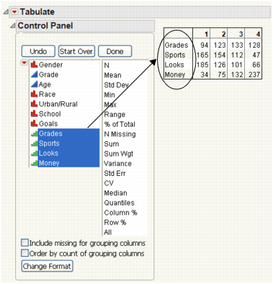
Example of Columns by Categories
1. Open the Children’s Popularity.jmp sample data table.
This data table contains data on the importance of self-reported factors in children’s popularity.
2. Select Tables > Tabulate.
3. Select Grades, Sports, Looks, and Money and drag and drop them into the Drop zone for rows.
4. Select Add Columns by Categories.
Figure 8.10 Columns by Categories
Tabulate the percentage of the one to four ratings of each category.
5. Drag and drop Gender into the empty heading at left.
6. Drag and drop % of Total above one of the numbered headings.
7. Drag and drop All above the number 4.
Figure 8.11 Tabulating the Percentages

Break down the tabulation further by adding demographic data.
8. Drag and drop Urban/Rural below the % of Total heading.
Figure 8.12 Adding Demographic Data
Click and Drag Items
Each column heading has two zones: the upper and the lower. As you drag each column heading into a zone, the cursor transforms into a rectangle to indicate that you can drop the column heading at that position.
• Dropping in the upper zone places the new items above (before) the items on which the addition is dropped.
• Dropping in the lower zone places the addition below (after) the items on which the addition is dropped.
Each row label has two zones: the left and the right:
• Dropping in the left zone puts the new items to the left (before) of the items dropped on.
• Dropping in the right zone puts them to the right (after) of the items dropped on.
Note: You can drag columns from the Table panel in the data table onto a Tabulate table instead of using the Tabulate Control Panel.
In a properly created table, all grouping columns are together, all analysis columns are together, and all statistics are together. Therefore, JMP does not intersperse a statistics keyword within a list of analysis columns. JMP also does not insert an analysis column within a list of grouping columns.
If the items’ role is obvious, such as keywords or character columns, when you drag and drop, JMP populates the table automatically with the given items. Otherwise, a popup menu lets you choose the role for the items. Roles included on the popup menu are:
Add Grouping Columns
Choose Add Grouping Columns if you want to use the variables to categorize the data. For multiple grouping columns, Tabulate creates a hierarchical nesting of the variable.
Add Analysis Columns
Choose Add Analysis Columns if you want to compute the statistics of these columns.
Columns by Categories
Choose Columns by Categories if the columns are independent grouping columns (in other words, no hierarchical nesting) sharing a similar set of distinct data values, and if you want a cross tabulation of the column by the categories layout.
Grouping Columns for Separate Tables
Choose Grouping Columns for Separate Tables if you have multiple independent grouping columns and you want to generate separate tables for each grouping column.
Insert a Grouping Column
To insert a grouping column, click and drag, and then release a column name or statistics keyword into the table. Select Add Grouping Columns from the menu that appears, as shown in Figure 8.13. If adding it as a grouping column is the only logical choice, JMP automatically inserts it as a grouping column; the popup menu does not appear.
Figure 8.13 Example of Adding a Grouping Column
Insert an Analysis Column
To insert an analysis column, click and drag, and then release a column name or statistics keyword into the table. Select Add Analysis Columns from the menu that appears, as shown in Figure 8.13.
Use the Dialog
If you prefer not to click and drag and build the table interactively, you can create a simple table using the Dialog interface. After selecting Tables > Tabulate, select Dialog from the drop-down menu beside Build table using, as shown in Figure 8.14. The window that appears is very similar to the Summary window, and the resultant table is like the layout of the summary table. (See Summarize Columns.) You can change the table generated by the window in the same way that you would with one generated through drag and drop.
Figure 8.14 Using the Window

Column Tables and Row Tables
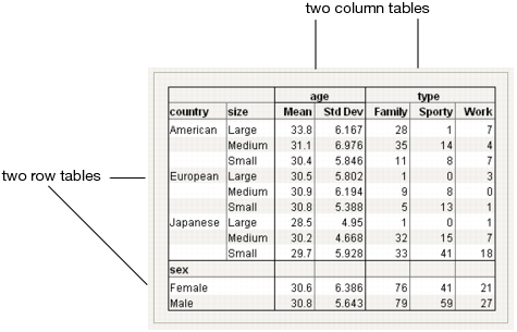
The Tabulate platform enables you to build sub-tables within a larger table. These sub-tables are called row tables and column tables, as illustrated in Figure 8.15 using Car Poll.jmp.
Example of Row and Column Tables
1. Open the Car Poll.jmp sample data table.
2. Select Tables > Tabulate.
3. Drag size into the Drop zone for rows.
4. Drag and drop country to the left of the size heading.
5. Drag and drop Mean over the N heading.
6. Drag and drop Std Dev below the Mean heading.
7. Drag and drop age above the Mean heading.
8. Select Add Analysis Columns.
9. Drag and drop type to the far right of the table.
10. Drag and drop sex under the table.
Figure 8.15 Row and Column Tables
Edit Tables in Tabulate
There are several ways to edit the items that you add to a table.
Change Numeric Formats
The formats of each cell depend on the analysis column and the statistics. For counts, the default format has no decimal digits. For each cell defined by some statistics, JMP tries to determine a reasonable format using the format of the analysis column and the statistics requested. To override the default format:
1. Click the Change Format button at the bottom of the Tabulate window.
2. In the panel that appears (Figure 8.16), enter the field width, a comma, and then the number of decimal places that you want displayed in the table.
3. (Optional) If you would like JMP to determine the best format for you to use, type the word Best in the text box.
JMP now considers the precision of each cell value and selects the best way to show it.
4. Click OK to implement the changes and close the Format section, or click Set Format to see the changes implemented without closing the Format section.
Figure 8.16 Changing Numeric Formats
Delete Items
After you add items to the table, you can remove them in any one of the following ways:
• Drag and drop the item away from the table.
• To remove the last item, click Undo.
• Right-click on an item and select Delete.
Remove Column Labels
Grouping columns display the column name atop the categories associated with that column. For some columns, the column name might seem redundant. Remove the column name from the column table by right-clicking on the column name and selecting Remove Column Label. To re-insert the column label, right-click on one of its associated categories and select Restore Column Label.
Edit Statistical Key Words and Labels
You can edit a statistical key word or a statistical label. For example, instead of Mean, you might want to use the word Average. To make edits, right-click on the word that you want to edit and select Change Item Label. In the box that appears, type the new label. Alternatively, you can type directly into the edit box.
If you change one statistics keyword to another statistics keyword, JMP assumes that you actually want to change the statistics, not just the label. It would be as if you have deleted the statistics from the table and added the latter.
Additional Tabulate Options
Tabulate options appear within the red triangle menu next to Tabulate and within the Control Panel.
Change Format
Enables you to change the numeric format for displaying specific statistics. See Change Numeric Formats.
Change Plot Scale
(Only appears if Show Chart is selected from the red triangle menu.) Enables you to specify a uniform custom scale.
Uniform plot scale
(Only appears if Show Chart is selected from the red triangle menu.) Deselect this box to have each column of bars use the scale determined separately from the data in each displayed column.
Include missing for grouping columns
Creates a separate group for missing values in grouping columns. When unchecked, missing values are not included in the table. Note that any missing value codes that you have defined as column properties are taken into account.
Order by count of grouping columns
Changes the order of the table to be in ascending order of the values of the grouping columns.
Other options are available from the red triangle menu next to Tabulate:
Show tool tip
Displays tips that appear when you move the mouse over areas of the table.
Show Shading
Displays gray shading boxes in the table when there are multiple rows.
Show Table
Displays the summarized data in tabular form.
Show Chart
Displays the summarized data in bar charts that mirrors the table of summary statistics. The simple bar chart enables visual comparison of the relative magnitude of the summary statistics. By default, all columns of bars share the same scale. You can have each column of bars use the scale determined separately from the data in each displayed column, by clearing the Uniform plot scale check box. You can specify a uniform custom scale using the Change Plot Scale button. The charts are either 0-based or centered on 0. If the data are all nonnegative, or all non-positive, the charts baseline is at 0. Otherwise, the charts are centered on 0.
Show Control Panel
Displays the control panel for further interaction.
Show Test Build Panel
Displays the control area that lets you create a test build using a random sample from the original table. See Use Large Amounts of Data (the Test Build Feature), for details.
Make Into Data Table
Makes a data table from the report. There is one data table for each row table, since labels of different row tables might not be mapped to the same structure.
Script
Displays options for saving scripts, redoing analyses, and viewing the data table. For details, see Save Your Analysis as a Script in Save and Share Data.
Use Large Amounts of Data (the Test Build Feature)
If you have a very large data table, you might want to use a small subset of the data table to try out different table layouts to find one that best shows the summary information. In this case, JMP generates a random subset of the size as specified and uses that subset when it builds the table. To use the test build feature:
1. From the red triangle menu next to Tabulate, select Show Test Build Panel.
2. Enter the size of the sample that you want in the box under Sample Size (>1) or Sampling Rate (<1), as shown in Figure 8.17. The size of the sample can be either the proportion of the active table that you enter or the number of rows from the active table.
Figure 8.17 The Test Build Panel
3. Click Resample.
4. To see the sampled data in a JMP data table, click the Test Data View button. When you dismiss the test build panel, Tabulate uses the full data table to regenerate the tables as designed.
Example of Tabulating Data
This example contains the following procedures:
Create a Table of Counts
Suppose you would like to view a table that contains counts for how many people in the survey own Japanese, European, and American cars.
1. Open the Car Poll.jmp sample data table.
2. Select Tables > Tabulate.
3. Click country and drag it into the Drop zone for rows.
Now add further statistics and variables to the table. You would like to see a count of people who drive Japanese, European, and American cars broken down by the size of the car.
4. Click size and drag and drop it to the right of the country heading.
Figure 8.18 Adding Size to the Table
Create a Table Showing Statistics
Now, suppose you would like to see the average and the standard deviation of the age of people who own each size car:
1. Start from Figure 8.18. Click age and drag and drop it to the right of the size heading.
2. Select Add Analysis Columns.
3. Click Mean and drag and drop it over Sum.
4. Click Std Dev and drag and drop it below Mean.
This places Std Dev below Mean in the table. Dropping Std Dev above Mean places Std Dev above Mean in the table.
Figure 8.19 Table that Includes the Mean and Standard Deviation of Age

Rearrange the Table Contents
To rearrange the table contents, proceed as follows:
1. Start from Figure 8.19. Click on the size heading and drag and drop it to the right of the table headings. See Figure 8.20.
Figure 8.20 Moving size
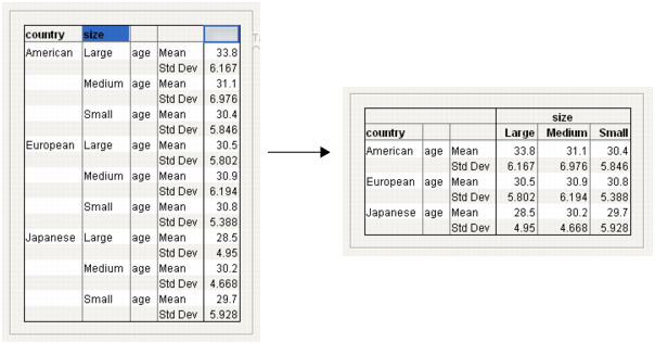
2. Click on age and drag and drop it under the Large heading.
3. Select both Mean and Std Dev, and then drag and drop them under the Large heading.
Figure 8.21 The Result of Moving Items

Now your table clearly presents the data. It is easy to see the mean and standard deviation of the car owner age broken down by car size and country.
..................Content has been hidden....................
You can't read the all page of ebook, please click here login for view all page.