Chapter 4

Regression and ANOVA Review

Regression

Simple Regression

Multiple Regression

Regression with Categorical Data

ANOVA

One-way ANOVA

Testing Statistical Assumptions

Testing for Differences

Two-way ANOVA

References

Simple and multiple regression and ANOVA, as shown in our multivariate analysis framework in Figure 4.1, are two dependence techniques that are most likely covered in an introductory statistics course. In this chapter, we will review these two techniques, illustrate the process of performing these analyses in JMP, and explain how to interpret the results.

Regression

One of the most popular applied statistical techniques is regression. Regression analysis typically has one of two main purposes. Either it is being used to understand the cause and effect relationship between one dependent variable and one or more independent variables. For example, how does the amount of advertising effect sales. Or regression is applied for prediction—in particular, for the purpose of forecasting a dependent variable based on one or more independent variables. An example would be using trend and seasonal components to forecast sales. Regression analyses can handle linear or nonlinear relationships, although the linear models are mostly emphasized.

Simple Regression

Let’s look at the data set salesperfdata.jmp. This data is from Cravens et al. (1972) and consists of the sales from 25 territories and seven corresponding variables:

■ Salesperson’s experience (Time)

■ Market potential (MktPoten)

■ Advertising expense (Adver)

■ Market Share (MktShare)

■ Change in Market Share (Change)

■ Number of accounts (Accts)

■ Workload per account (WkLoad)

Figure 4.1  A Framework to Multivariate Analysis

First, we will do only a simple linear regression, which is defined as one dependent variable Y and only one independent variable X. In particular, let’s look at how advertising is related to sales:

Open the salesperfdata.jmp in JMP. Select Analyze→Fit Y by X. In the Fit Y by X dialog box, click Sales and click Y, Response. Click Adver and click X, Factor. Click OK.

A scatterplot of sales versus advertising, similar to Figure 4.2 (without the red line), will appear. There appears to be a positive relationship, which means that as advertising increases, sales increase. To further examine and evaluate this relationship: Click the red triangle and click Fit Line. Fit Line causes the creation of the tables that contain the regression results. A simple linear regression is performed. The output will look like the bottom half of Figure 4.2. The regression equation is: Sales = 2106.09 + 0.2911*Adver. The y-intercept (black) and Adver (red) coefficient values are identified in Figure 4.2 under Parameter Estimates.

The F-test and t-test, in simple linear regression, are equivalent in that they both test whether the independent variable (Adver) is significantly related to the dependent variable (Sales). As indicated in Figure 4.2, both p-values are equal to 0.0017 and are significant. (To assist you in identifying significant relationships, JMP puts an asterisk next to a p-value that is significant with α = 0.05.) This model’s goodness-of-fit is measured by the coefficient of determination (R² or RSquare) and the standard error (s_e or Root Mean Square Error), which in this case is equal to 35.5% and 1076.87, respectively.

Figure 4.2  Scatterplot with Corresponding Simple Linear Regression

Multiple Regression

We will next examine the multiple linear regression relationship between sales and the seven predictors (Time, MktPoten, Adver, MktShare, Change, Accts, and WkLoad), which is equivalent to those used by Cravens et al. (1972). Before performing the multiple linear regression, let’s first examine the correlations and scatterplot matrix:

Select Analyze→Multivariate Methods→Multivariate. In the Multivariate and Correlations dialog box, in the Select Columns box, click Sales, hold down the shift key, and click WkLoad. Click Y,Columns, and all the variables will appear in the white box to the right of Y, Columns, as in Figure 4.3. Click OK.

Figure 4.3  The Multivariate and Correlations Dialog Box

As shown in Figure 4.4, the correlation matrix and corresponding scatterplot matrix will be generated. Examine the first row of the Scatterplot Matrix. There appear to be several strong correlations, especially with the dependent variable Sales. All the variables, except for Wkload, have a strong positive relationship (or positive correlation) with Sales. The oval shape in each scatterplot is the corresponding bivariate normal density ellipse of the two variables. If the two variables are bivariate normally distributed, then, about 95% of the points would be within the ellipse. If the ellipse is rather wide (round) and does not follow either of the diagonals, then the two variables do not have a strong correlation. For example, observe the ellipse in the scatterplot for Sales and Wkload and notice that the correlation is -0.1172. The more significant the correlation, the more narrow the ellipse, and the more it follows along one of the diagonals (for example Sales and Accts).

To perform the multiple regression:

Select Analyze→Fit Model. In the Fit Model dialog box, as shown in Figure 4.5, click Sales and click Y. Next, click Time, hold down the shift key, and click WkLoad. Now all the independent variables from Time to WkLoad are highlighted. Click Add and now these independent variables are listed. Notice the box to the right of Personality. It should say Standard Least Squares. Click the drop-down arrow to the right and observe the different options, which include stepwise regression (which we will discuss later in the chapter). Keep it at Standard Least Squares and click Run.

Figure 4.4  Correlations and Scatterplot Matrix for the salesperfdata.jmp data

Figure 4.5  The Fit Model Dialog Box

As shown in Figure 4.6, the multiple linear regression equation is:

Sales = -1485.88 + 1.97*Time + 0.04*MktPoten + 0.15*Adver + 198.31

*MktShare + 295.87*Change + 5.61* Accts +19.90*WkLoad.

Each independent variable regression coefficient represents an estimate of the change in the dependent variable that, in turn, corresponds to a unit increase in that independent variable while all the other independent variables are held constant. For example, the coefficient for WkLoad is 19.9. If WkLoad is increased by 1 and the other independent variables do not change, then Sales would correspondingly increase by 19.9.

The relative importance of each independent variable is measured by its standardized beta coefficient (which is a unitless value). The larger the absolute value of the standardized beta coefficient, the more important the variable. To obtain the standardized beta values, move the cursor somewhere over the Parameter Estimates Table and right-click. A list of options will appear, including Columns. Select Columns→Std Beta. Subsequently, the Std Beta column is added to the Parameter Estimates Table, as shown in Figure 4.7. With our sales performance data set, we can see that the variables MktPoten, Adver, and MktShare are the most important variables.

Figure 4.6  Multiple Linear Regression Output

Figure 4.7  Parameter Estimates Table with Standardized Betas and VIFs

The steps to evaluate a multiple regression model are listed in Figure 4.8. First, you should perform an F-test. The F-test, in multiple regression, is known as an overall test.

Figure 4.8  Steps to Evaluating a Regression Model

The hypotheses for the F-test are:

; where k is the number of independent variables.

If we fail to reject the F-test, then the overall model is not statistically significantly. The model shows no linear significant relationships. We need to start over, and we should not look at the numbers in the Parameter Estimates table. On the other hand, if we reject H₀ of the F-test, then we can conclude that one or more of the independent variables are linearly related to the dependent variable. So we want to reject H₀ of the F-test.

In Figure 4.6, for our sales performance data set, we can see that the p-value for the F-test is <0.0001. So we reject the F-test and can conclude that one or more of the independent variables (i.e., one or more of variables Time, Mktpoten, Adver, Mktshare, Change, Accts, and Wkload) is significantly related to Sales (linearly).

The second step is to evaluate the t-test for each independent variable. Even though the hypotheses are:

we are not testing whether independent variable k, x_k, is significantly related to the dependent variable. What we are testing is whether x_k is significantly related to the dependent variable above and beyond all the other independent variables that are currently in the model. That is, in the regression equation, we have the term . If , then x _k has no effect on Y. Again, we want to reject H ₀. We can see in Figures 4.6 and 4.7 that the independent variables MktPoten, Adver, and MktShare each reject H₀ and are significantly related to Sales above and beyond the other independent variables.

One of the statistical assumptions of regression is that the residuals or errors (the difference between the actual value and the predicted value) should be random. That is, the errors do not follow any pattern. To visually examine the residuals, you can produce a plot of the residuals versus the predicted values by clicking the red triangle and selecting Row Diagnostics→Plot Residual by Predicted. A graph similar to Figure 4.9 will appear. Examine the plot for any patterns—oscillating too often or increasing or decreasing in values or for outliers. The data in Figure 4.9 appears to be random.

Figure 4.9  Residual Plot of Predicted versus Residual

If the observations were taken in some time sequence, called a time series (not applicable to our sales performance data set), the Durbin-Watson test should be performed (click the red triangle next to the Response Sales heading; select Row Diagnostics→Durbin-Watson Test). To display the associated p-value, click the red triangle under the Durbin-Watson test and click Significant p-value. The Durbin-Watson test examines the correlation between consecutive observations. (In this case, you want high p-values; high p-values of the Durbin-Watson test indicate that there is no problem with first order autocorrelation.)

An important problem to address in the application of multiple regression is multicollinearity or collinearity of the independent variables (Xs) as in step 4 in Figure 4.8. Multicollinearity occurs when the two or more independent variables explain the same variability of Y. Multicollinearity does not violate any of the statistical assumptions of regression. However, significant multicollinearity is likely to make it difficult to interpret the meaning of the regression coefficients of the independent variables.

One method of measuring multicollinearity is the variance inflation factor (VIF). Each independent variable k has its own VIF_k. By definition, it must be greater than or equal to 1. The closer the VIF_k is to 1, the smaller the relationship between the kth independent variable and the remaining Xs. Although, there are no definitive rules for identifying a large VIF_k, the basic guidelines (Marquardt, 1980) (Snee, 1973) for identifying whether significant multicollinearity exists are:

1 ≤ VIF_k ≤ 5   no significant multicollinearity

5 < VIF_k ≤ 10   be concerned that some multicollinearity may exist

VIF_k > 10   significant multicollinearity

Note: Exceptions to these guidelines are when you may have transformed the variables (such as nonlinear transformation). To display the VIF_k values for the independent variables (similar to what we illustrated to display the standardized beta values), move the cursor somewhere over the Parameter Estimates Table and right-click. Select Columns→VIF. As shown before in Figure 4.7, a column of VIF values for each independent variable is added to the Parameter Estimate Table. The variable Accts has a VIF greater than 5, and we should be concerned about that variable.

There are two opposing point of views as to whether to include those non-significant independent variables (i.e., those variables for which we failed to reject H₀ for the t-test) or the high VIF_k variables. One perspective is to include those non-significant/high VIF_k variables because they explain some, although not much, of the variation in the dependent variable, and it does improve your understanding of these relationships. Taking this approach to the extremes, you can keep on adding independent variables to the model so that you have almost the same number of independent variables as there are observations, which is somewhat unreasonable. However, this approach is sensible with a reasonable number of independent variables and if the major objective of the regression analysis is understanding the relationships of the independent variables to the dependent variable. Nevertheless, addressing the high VIF_k values (especially > 10) may be of concern, particularly if one of the objectives of performing the regression is the interpretation of the regression coefficients.

The other point of view follows the principle of parsimony, which states that the smaller the number of variables in the model, the better. This viewpoint is especially true when the regression model is used for prediction/forecasting (having such variables in the model may actually increase the s_e). There are numerous approaches and several statistical variable selection techniques to achieve this goal of only significant independent variables in the model. Stepwise regression is one of the simplest approaches. Although it’s not guaranteed to find the “best” model, it certainly will provide a model that is close to the ‘best.” To perform stepwise regression, we have two alternatives:

1. Click the red triangle next to the Response Sales heading and select Model Dialog. The Fit Model dialog box as in Figure 4.5 will appear.

2. Select Analyze→Fit Model. Click the Recall icon. The dialog box is repopulated and looks like Figure 4.5.

In either case, now, in the Fit Model dialog box, click the drop-down arrow to the right of Personality. Change Standard Least Squares to Stepwise. Click Run.

The Fit Stepwise dialog box will appear, similar to the top portion of Figure 4.10. In the drop-down box to the right of Stopping Rule, click the drop-down arrow, and change the default from Minimum BIC to P-Value Threshold. Two rows will appear, Prob to Enter and Prob to Leave. Change Direction to Mixed. (The Mixed option alternates the forward and backward steps.) Click Go.

Figure 4.10 displays the stepwise regression results. The stepwise model did not include the variables Accts and Wkload. The Adjusted R² values improved slightly from 0.890 in the full model to 0.893; and the s_e (or Root Mean Square Error (RMSE)) actually improved by decreasing from 435.67 to 430.23. And nicely now, all the p-values for the t-tests are now significant (less than 0.05).

Figure 4.10  Stepwise Regression for the Sales Performance Data Set

How good of a fit the regression model is measured by the Adjusted R² and the s_e or RMSE, as listed in Figure 4.8. The Adjusted R² measures the percentage of the variability in the dependent variable that is explained by the set of independent variables and is adjusted for the number of independent variables (Xs) in the model. If the purpose of performing the regression is to understand the relationships of the independent variables with the dependent variable, the Adjusted R² value is a major assessment of the goodness of fit. What constitutes a good Adjusted R² value is subjective and depends on the situation. The higher the Adjusted R², the better the fit. On the other hand, if the regression model is for prediction/forecasting, the value of the s_e is of more concern. A smaller s_e generally means a smaller forecasting error. Similar to Adjusted R², a good s_e value is subjective and depends on the situation.

Two additional approaches to consider in the model selection process that do consider both the model fit and the number of parameters in the model are the information criterion (AIC) approach developed by Akaike and the Bayesian information criterion (BIC) developed by Schwarz. The two approaches have quite similar equations except that the BIC criterion imposes a greater penalty on the number of parameters than the AIC criterion. Nevertheless, in practice, the two criteria often produce identical results. To apply these criteria, in the Stepwise dialog box when you click the drop-down arrow for Stopping Rule there were several options listed, including Minimum AICc and Minimum BIC.

Regression with Categorical Data

There are many situations in which a regression model that uses one or more categorical variable(s) as (an) independent variable(s) may be of interest. For example, let’s say our dependent variable is sales. A few possible illustrations of using a categorical variable that could affect sales would be gender, region, store, or month. The goal of using these categorical variables would be to see if the categorical variable may or may not significantly affect the dependent variable sales. That is, does the amount of sales differ significantly by gender, by region, by store, or by month? Or do sales vary significantly in combinations of several of these categorical variables?

Measuring ratios and distances are not appropriate with categorical data. That is, distance cannot be measured between male and female. So in order to use a categorical variable in a regression model, we must transform the categorical variable(s) into (a) continuous variable(s) or (an) integer (binary) variable(s). The resulting variables from this transformation are called indicator or dummy variables. How many indicator/dummy variables are required for a particular independent categorical variable X is equal to c-1, where c is the number of categories (or levels) of the categorical X variable. For example, gender requires one dummy variable, and month requires 11 dummy variables. In many cases, the dummy variables are coded 0 or 1. However, in JMP this is not the case. If a categorical variable has two categories (or levels) such as gender, then a single dummy variable is used with values of +1 and -1 (with +1 assigned to the alphabetically first category). If a categorical variable has more than two categories (or levels), the dummy variables are assigned values +1, 0 and -1.

Let’s look at a data set, in particular AgeProcessWords.jmp (Eysenck, 1974). Eysenck conducted a study to examine whether age and the amount remembered is related to how the information was initially processed. Fifty younger and fifty older people were randomly assigned to five learning process groups (Counting, Rhyming, Adjective, Imagery, and Intentional), where younger was defined as being younger than 54 years old. The first four learning process groups were instructed on ways to memorize the 27 items. For example, the rhyming group was instructed to read each word and think of a word that rhymed with it. These four groups were not told that they would later be asked to recall the words. On the other hand, the last group, the intentional group, was told that they would be asked to recall the words. The data set has three variables: Age, Process, and Words.

To run a simple regression using the categorical variable Age to see how it is related to the number of words memorized, the variable Words:

Select Analyze→Fit Model. In the Fit Model dialog box, select Words→Y. Then select Age→Add. Click Run.

Figure 4.11 shows the regression results. We can see from the F-test and t-test that Age is significantly related to Words. The regression equation is: Words = 11.61 -1.55*Age[Older].

As we mentioned earlier, with a categorical variable with two levels, JMP assigns +1 to the alphabetically first level and -1 to the other level. So in this case, Age[Older] is assigned +1 and Age[Younger] is assigned -1. So the regression equations for each Age group are:

Older Age group: Words = 11.61 -1.55*Age[Older] = 11.61 -1.55(1) = 10.06

Younger Age group: Words = 11.61 -1.55*Age[Older] = 11.61 -1.55(-1) = 13.16

Therefore, the Younger age group can remember more words.

To verify the coding (and if you wish to create a different coding in other situations), we can create a new variable called Age1 by:

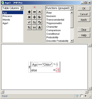
Select Cols→New Columns. The new column dialog box will appear. In the text box for Column name, where Column 4 appears, type Age1. Click the drop-down arrow for Column Properties, and click Formula. The Formula dialog box will appear. In the text box below on the right for Functions (Grouped), select Conditional→If. The If statement will appear in the formula area. JMP has placed the cursor on expr (red rectangle). Click Age from the Table Columns. In the text box below on the right for Functions (Grouped), click Comparison>a==b. In the new red rectangle, type “Older” (include quotation marks), and then press the Tab key. Click on the top then clause, type 1, and then press the Tab key again. Double-click on the lower else clause and type −1. The dialog box should look like Figure 4.12. Click OK and then click OK again.

Figure 4.11  Regression of Age on Number of Words Memorized 

Figure 4.12  Formula Dialog Box 

A new column Age1 with +1s and −1s will be in the data table. Now, we run a regression with Age1 as the independent variable. Figure 4.13 displays the results. Comparing the results in Figure 4.13 to the results in Figure 4.11, we see that they are exactly the same.

A regression that examines the relationship between Words and the categorical variable Process would use four dummy variables.

Select Analyze→Fit Model. In the Fit Model dialog box, select Process→Y. Select Age→Add. Click Run.

Figure 4.13  Regression of Age1 on Number of Words Memorized 

Figure 4.14  Dummy Variable Coding for Process and the Predicted Number of Words Memorized

Row Process	Predicted # of Words	Process Dummy Variable
		[Adjective]	[Counting]	[Imagery]	[Intentional]
Adjective	12.9	1	0	0	0
Counting	6.75	0	1	0	0
Imagery	15.5	0	0	1	0
Intentional	15.65	0	0	0	1
Rhyming	7.25	-1	-1	-1	-1

Figure 4.15  Regression of Process on Number of Words Memorized

The coding used for these four Process dummy variables is shown in Figure 4.14. Figure 4.15 displays the regression results. The regression equation is:

Words = 11.61 +1.29*Adjective – 4.86*Counting + 3.89*Imagery + 4.04*Intentional

Given the dummy variable coding used by JMP, as shown in Figure 4.14, the mean of the level displayed in the brackets is equal to the difference between its coefficient value and the mean across all levels (that is, the overall mean or the y-intercept). So the t-tests here are testing if the level shown is different from the mean across all levels. If we haved used the dummy variable coding and substituted into the equation, the predicted number of Words that are memorized by process are as listed in Figure 4.14. Intentional has the highest words memorized at 15.65, and Counting is the lowest at 6.75.

ANOVA

Analysis of variance (more commonly called ANOVA), as shown in Figure 4.1, is a dependence multivariate technique. There are several variations of ANOVA, such as one-factor (or one-way) ANOVA, two-factor (or two-way) ANOVA, and so on, and also repeated measures ANOVA. (In JMP, repeated measures ANOVA is found under Analysis→Modeling→Categorical.) The factors are the independent variables, each of which must be a categorical variable. The dependent variable is one continuous variable. We will provide only a brief introduction/review to ANOVA.

Let’s assume one independent categorical variable X has k levels. One of the main objectives of ANOVA is to compare the means of two or more populations, i.e.:

.

The average for each level is µ_k. If H₀ is true, we would expect all the sample means to be close to each other and relatively close to the grand mean. If H₁ is true, then at least one of the sample means would be significantly different. We measure the variability between means with the sum of squares between groups (SSBG). On the other hand, large variability within the sample weakens the capacity of the sample means to measure their corresponding population means. This within-sample variability is measured by the sum of squares within groups (or error) (SSE). As with regression, the decomposition of the Total sum of squares (TSS) is equal to:

Total Sum of Squares = Sum of Squares Between Groups + Sum of Squares Error or

TSS = SSBG + SSE.

(In JMP: TSS, SSBG, and SSE are identified as C.Total, Model SS, and Error SS, respectively.) To test this hypothesis, we do an F-test (the same as what is done in regression).

If H₀ of the F-test is rejected, which implies that one or more of the population means are significantly different, we then proceed to the second part of an ANOVA study and identify which factor level means are significantly different. If we have two populations (that is, two levels of the factor), we would not need ANOVA and we could perform a two-sample hypothesis test. On the other hand, when we have more than two populations (or groups) we could take the two-sample hypothesis test approach and compare every pair of groups. This approach has problems that are caused by multiple comparisons and is not advisable, as we will explain. If there are k levels in the X variable, the number of possible pairs of levels to compare is k(k-1)/2. For example, if we had three populations (call them A, B, and C), there would be 3 pairs to compare: A to B, A to C, and B to C. If we use a level of significance α = 0.05, there is a 14.3% (1-(.95)³) chance that we will detect a difference in one of these pairs, even when there really is no difference in the populations; the probability of Type I error is 14.3%. If there are 4 groups, the likelihood of this error increases to 26.5%. This inflated error rate for the group of comparisons, not the individual comparisons, is not a good situation. However, ANOVA provides us with several multiple comparison tests that maintain the Type I error at α or smaller.

An additional plus of ANOVA is, if we are examining the relationship of two or more factors, ANOVA is good at uncovering any significant interactions or relationships among these factors. We will discuss interactions briefly when we examine two-factor (two-way) ANOVA. For now, let’s look at one-factor (one-way) ANOVA.

One-way ANOVA

One-way ANOVA has one dependent variable and one-X factor. Let’s return to the AgeProcessWords.jmp data set and first perform a one-factor ANOVA with Words and Age:

Select Analyze→Fit Y by X. In the Fit Y by X dialog box, select Words→Y, Response. Select Age→X, Factor. Click OK. In the Fit Y by X output, click the red triangle and select the Means/Anova/Pooled t option.

Figure 4.16 displays the one-way ANOVA results. The plot of the data at the top of Figure 4.16 is displayed by each factor level (in this case, the age group Older and Younger). The horizontal line across the entire plot represents the overall mean. Each factor level has its own mean diamond. The horizontal line in the center of the diamond is the mean for that level. The upper and lower vertices of the diamond represent the upper and lower 95% confidence limit on the mean, respectively. Additionally, the horizontal width of the diamond is relative to that level’s (group’s) sample size; that is, the wider the diamond, the larger the sample size for that level relative to the other levels. In this case, because the level sample sizes are the same, the horizontal widths of all the diamonds are the same. As shown in Figure 4.16, the t-test and the ANOVA F-test (in this situation, since the factor Age has only two levels, a pooled t-test is performed) show that there is a significant difference in the average Words memorized by Age level (p = 0.0024). In particular, examining the Means for Oneway ANOVA table in Figure 4.16, we can see that the Younger age group memorizes more words than the Older group (average of 13.16 to 10.06). Lastly, compare the values in the ANOVA table in Figure 4.16 to Figures 4.11 and 4.13. They have exactly the same values in the ANOVA tables when we did the simple categorical regression using AGE or AGE1.

Figure 4.16 One-way ANOVA of Age and Words

Testing Statistical Assumptions

ANOVA has three statistical assumptions to check and address. The first assumption is that the residuals should be independent. In most situations, ANOVA is rather robust in terms of this assumption. Furthermore, many times in practice this assumption is violated. So unless there is strong concern about the dependence of the residuals, this assumption does not have to be checked.

The second statistical assumption is that the variances for each level are equal. Violation of this assumption is of more concern because it could lead to erroneous p-values and hence incorrect statistical conclusions. We can test this assumption by clicking the red triangle and then clicking Unequal Variances. Added to the JMP ANOVA results is the Tests that the Variances are Equal report. Four tests are always provided. However, if, as it is in this case, there are only two groups tested, then an F-test for unequal variance is also performed; this gives us five tests, as shown in Figure 4.17. If we fail to reject H₀ (that is, we have a large p-value), we have insufficient evidence to say that the variances are not equal. So we proceed as though they are equal. On the other hand, if we reject H₀, the variances can be assumed to be unequal, and the ANOVA output cannot be trusted. For our problem, because for all the tests for unequal variances, the p-values are small, we need to look at the Welch’s Test, located at the bottom of Figure 4.17. The p-value for the Welch ANOVA is 0.0025, which is also rather small. So we can assume that there is a significant difference in the population mean of Older and Younger.

The third statistical assumption is that the residuals should be normally distributed. The F-test is very robust if the residuals are non-normal. That is, if slight departures from normality are detected, they will have no real effect on the F statistic. A normal quantile plot can confirm whether the residuals are normally distributed or not. To produce a normal quantile plot:

In the Fit Y by X output, click the red triangle and select Save→Save residuals. A new variable called Words centered by Age will appear in the data table. Select Analyze→Distribution. In the Distribution dialog box, in the Select Columns area, select Words centered by Age→ Y, Response. Click OK. The Distribution output will appear. Click on the middle red triangle (next to Words centered by Age), and click Normal Quantile Plot.

Figure 4.17  Tests of Unequal Variances and Welch’s Test for Age and Words

The distribution output and normal quantile plot will look like Figure 4.18. If all the residuals fall on or near the straight line or within the confidence bounds, the residuals should be considered normally distributed. All the points in Figure 4.18 are within the bounds, so we can assume that the residuals are normally distributed.

Figure 4.18  Normal Quantile Plot of the Residuals

Let’s now perform a one-factor ANOVA of Process and Words:

Figure 4.19  One-way ANOVA of Process and Words

Select Analyze→Fit Y by X. In the Fit Y by X dialog box, select Words→Y, Response. Select Process→X, Factor. Click OK. Click the red triangle and click Means/Anova.

Figure 4.19 displays the one-way ANOVA results. The p-value for the F-test is <0.0001, so one or more of the Process means differ from each other. Also, notice that the ANOVA table in Figure 4.19 is the same as in the categorical regression output of Words and Process in Figure 4.15. The results of the tests for unequal variances are displayed in Figure 4.20.

Figure 4.20  Tests of Unequal Variances and Welch’s Test for Process and Words

In general, the Levene test is more widely used and more comprehensive, so, we focus only on the Levene test. It appears that we should assume that the variances are unequal (for all the tests), so we should look at the Welch’s Test in Figure 4.20. Because the p-value for the Welch’s Test is small, we can reject the null hypothesis; the pairs of means are different from one another.

Testing for Differences

The second part of the ANOVA study focuses on identifying which factor level means differ from each other. However, with the AgeProcessWords.jmp data set, because we did not satisfy the statistical assumption that the variances for each level are equal, we will not perform the second stage of the ANOVA study with that data set. (In general, it is not recommended to perform these second stage tests if the equal variances assumption is not satisfied. Nonetheless, if you do, JMP does provide some nonparametric tests.)

Consequently, let’s use another data set, Analgesics.jmp. The Analgesics data table contains 33 observations and three variables, Gender, Drug (3 analgesics drugs: A, B, and C), and Pain (ranges from 2.13 and 16.64—in which the higher the value, the more painful). Figures 4.21 and 4.22 display the two one-way ANOVAs. Males appear to have significantly higher Pain, and there does seem to be significant differences in Pain by Drug. The p-value for the Levene test is 0.0587, so we fail to reject the null hypothesis of all equal variances and can comfortably move on to the second part of an ANOVA study. (On the other hand, in Figure 4.22 the diamonds under Oneway analysis of pain by Drug appear different, suggesting possible different variances. If we select the red triangle and click Unequal Variances, we can check the Welch’s Test. Since the p-value for the Welch’s Test is small, we can reject the null hypothesis; the pairs of means are different from one another.)

Figure 4.21  One-way ANOVA of Gender and Pain

Figure 4.22  One-way ANOVA of Drug and Pain 

JMP provides several multiple comparison tests, which can be found by clicking the red triangle, clicking Compare Means, and then selecting the test. The first test, the Each Pair, Student’s t-test, computes individual pairwise comparisons. As discussed earlier, the likelihood of a Type I error increases with the number of pairwise comparisons. So, unless the number of pairwise comparisons is small, we do not recommend using this test.

The second means comparison test is the All Pairs, Tukey HSD test. If the main objective is to check for any possible pairwise difference in the mean values, and there are several factor levels, the Tukey HSD (Honestly Significant Difference) or Tukey-Kramer HSD test is the most desired test. Figure 4.23 displays the results of the Tukey-Kramer HSD test. To identify mean differences, examine the Connecting Letters Report. Groups that do not share the same letter are significantly different from one another. The mean pain for Drug A is significantly different from the mean pain of Drug C.

Figure 4.23  The Tukey-Kramer HSD Test

The third means comparison test is With Best, Hsu MCB. The Hsu’s MCB (multiple comparison with best) is used to determine whether each factor level mean can be rejected or not as the “best” of all the other means, where “best” means either a maximum or minimum value. Figure 4.24 displays the results of Hsu’s MCB test. The p-value report and the maximum and minimum LSD (Least Squares Differences) matrices can be used to identify significant differences. The p-value report identifies whether a factor level mean is significantly different from the maximum and from the minimum of all the other means. The Drug A is significantly different from the maximum, and Drugs B and C are significantly different from the minimum. The maximum LSD matrix compares the means of the groups against the unknown maximum and correspondingly the same for the minimum LSD matrix. Follow the directions below each matrix, looking at positive values for the maximum and negative values for the minimum.

Figure 4.24  The Hsu’s MCB Test

Examining the matrices in Figure 4.24, we can see that the Drug groups AC and AB are significantly less than the maximum and significantly greater than the minimum.

Differences with the Hsu’s MCB test are less conservative than those found with the Tukey-Kramer test. Additionally, Hsu’s MCB test should be used if there is a need to make specific inferences about the maximum or minimum values.

The last means comparison test provided, the with Control, Dunnett’s, is applicable when you do not wish to make all pairwise comparisons, but rather only to compare one of the levels (the “control”) with each other level. Thus, fewer pairwise comparisons are made. Because this is not a common situation, we will not discuss this test further.

In addition, one-way ANOVA can also be performed using the JMP Fit Model platform. Most of the output is identical to the Fit Y by X results, but, with a few differences. Let’s perform a one-way ANOVA on Pain with Drug:

Select Analyze→Fit Model. In the Fit Model dialog box, click Pain→Y. Select Drug→Add. Click Run. On the right side of the output, click the red triangle next to Drug and select LSMeans Plot→LSMeans Tukey HSD.

The output will look similar to Figure 4.25. Realize that these results are also equivalent to the regression results with these categorical variables that we discussed early in this chapter (see Figure 4.15). The LSMeans plot shows a plot of the factor means. The LSMeans Tukey HSD is similar to the All Pairs, Tukey HSD output from the Fit Y by X option. In Figure 4.25 and Figure 4.23, notice the same Connecting Letters Report. The Fit Model output does not have the LSD matrices but does provide us with a crosstab report. The Fit Model platform does not directly provide an equal variance test. But, you can visually evaluate the Residual by Predicted Plot in the lower left corner of Figure 4.25.

Figure 4.25  One-way ANOVA Output Using Fit Model

Two-way ANOVA

Two-way ANOVA is an extension of the one-way ANOVA in which there is one continuous dependent variable, but, now we have two categorical independent variables. There are three basic two-way ANOVA designs: without replication; with equal replication, and; with unequal replication. The two two-way designs with replication not only allow us to address the influence of each factor’s contribution to explaining the variation in the dependent variable, but, also allow us to address the interaction effects due to all the factor level combinations. We will only discuss the two-way ANOVA with equal replication.

Using the Analgesics.jmp, let’s perform a two-way ANOVA of Pain with Gender and Drug as independent variables:

Select Analyze→Fit Model. In the Fit Model dialog box, select Pain→Y. Click Gender, hold down the shift key, and click Drug. Then click Add. Again, click Gender, hold down the shift key, and click Drug. This time, click Cross. (Another approach: highlight Gender and Drug, click Macros, and click Full Factorial.) Click Run.

Figure 4.26 displays the two-way ANOVA results. The p-value for the F-test in the ANOVA table is 0.0006, so there are significant differences in the means. To find where the differences are, we examine the F-tests in the Effect Tests table. We can see that there are significant differences in the Age, Drug (which we found out already when we did the one-way ANOVAs). But we observe a moderately significant difference in the interaction means, p-value = 0.0916. To understand these differences, go back to the top of the output and click the red triangles for each factor and then:

For Gender: Select LSMeans Plot→LSMeans Student’s t (since we have only two levels).

For Drug: Select LSMeans Plot→LSMeans Tukey HSD.

For Gender*Drug: Select LSMeans Plot→LSMeans Tukey HSD.

The results for Gender and Drug displayed in Figure 4.26 are equivilant to what we observed earlier in the chapter when we discussed one-way ANOVA. Figure 4.27 also has the LSMeans Plot and the Connecting Letter Report for the interaction effect Gender*Drug. If there were no significant interaction, the lines in the LSMeans Plot would not cross and will be mostly parallel.

Figure 4.26  Two-way ANOVA Output

Figure 4.27  Two-way ANOVA Output for Gender, Drug, and Gender*Drug

This is not the case here. The Connecting Letter Report identifies further the significant interactions. Overall, and clearly in the LS Means Plot, it appears that Females have lower Pain than Males. However, for Drug A, Females have higher than expected Pain.

To check for equal variances in two-way ANOVA, we need to create a new column that is the interaction, Gender*Drug, and then run a one-way ANOVA on that variable. To create a new column when both variables are characters:

Select Cols→New Columns. The new column dialog box will appear. In the text box for Column name, where Column 4 appears, type Gender*Drug. Click the drop-down arrow for Column Properties and click Formula. The Formula dialog box will appear. Click the drop-down arrow next to Functions (Grouped), and click Functions (all). Scroll down until you see Concat and click it. The Concat statement will appear in the formula area with two rectangles. JMP has placed the cursor on the left rectangle (red rectangle). Click Gender from the Table Columns; click the right Concat rectangle and click Drug from the Table Columns. The dialog box should look like Figure 4.28. Click OK and then Click OK again.

Figure 4.28  Formula Dialog Box

The results of running a one-way ANOVA of Gender*Drug and Pain is shown in Figure 4.29. The F-test rejects the null hypothesis. So, as we have seen before, there is significant interaction.

Figure 4.29  One-way ANOVA with Pain and Interaction Gender*Drug

Examining the Levene test for equal variances, we have a p-value of 0.0084 rejecting the null hypothesis of all variances being equal. However, the results show a warning that the sample size is relatively small. So, in this situation, we will disregard these results.

References

Cravens, D. W., R. B. Woodruff, and J. C. Stamper. (January 1972). “An Analytical Approach for Evaluating Sales Territory Performance.” Journal of Marketing, Vol. 36, No. 1, 31–37.

Eysenck, M.W. (1974). Age differences in incidental learning. Developmental Psychology, Vol. 10, No. 6, 936–941.

Marquardt, D.W. (1980). “You Should Standardize the Predictor Variables in Your Regression Models.” Discussion of “A Critique of Some Ridge Regression Methods,” by G. Smith and F. Campbell. Journal of the American Statistical Association, Vol. 75, No. 369, 87–91.

Snee, R. D. (1973). “Some Aspects of Nonorthogonal Data Analysis: Part I. Developing Prediction Equations.” Journal of Quality Technology, Vol. 5, No. 2, 67–79.