Chapter 5

Logistic Regression 

Dependence Technique: Logistic Regression

The Linear Probability Model (LPM)

The Logistic Function

Example: toylogistic.jmp

Odds Ratios in Logistic Regression

A Logistic Regression Statistical Study

References

Exercises

Figure 5.1  A Framework for Multivariate Analysis

Dependence Technique: Logistic Regression

Logistic regression, as shown in our multivariate analysis framework in Figure 5.1, is one of the dependence techniques in which the dependent variable is discrete and, more specifically, binary. That is, it takes on only two possible values. Here are some examples: Will a credit card applicant pay off a bill or not? Will a mortgage applicant default? Will someone who receives a direct mail solicitation respond to the solicitation? In each of these cases, the answer is either “yes” or “no.” Such a categorical variable cannot directly be used as a dependent variable in a regression. But a simple transformation solves the problem: Let the dependent variable Y take on the value 1 for “yes” and 0 for “no.”

Because Y takes on only the values 0 and 1, we know E[Y_i] = 1*P[Y_i=1] + 0*P[Y_i=0] = P[Y_i=1] . But from the theory of regression, we also know that E[Y_i] = a + b*X_i. (Here we use simple regression, but the same holds true for multiple regression.) Combining these two results, we have P[Y_i=1] = a + b*X_i. We can see that, in the case of a binary dependent variable, the regression may be interpreted as a probability. We then seek to use this regression to estimate the probability that Y takes on the value 1. If the estimated probability is high enough, say above 0.5, then we predict 1; conversely, if the estimated probability of a 1 is low enough, say below 0.5, then we predict 0.

The Linear Probability Model (LPM)

When linear regression is applied to a binary dependent variable, it is commonly called the Linear Probability Model (LPM). Traditional linear regression is designed for a continuous dependent variable, and is not well-suited to handling a binary dependent variable. Three primary difficulties arise in the LPM. First, the predictions from a linear regression do not necessarily fall between zero and one. What are we to make of a predicted probability greater than one? How do we interpret a negative probability? A model that is capable of producing such nonsensical results does not inspire confidence.

Second, for any given predicted value of y (denoted ), the residual (resid= y - ) can take only two values. For example, if = 0.37, then the only possible values for the residual are resid= -0.37 or resid = 0.63 (= 1 – 0.37), because it has to be the case that + resid equals zero or one. Clearly, the residuals will not be normal. Plotting a graph of versus resid will produce not a nice scatter of points, but two parallel lines. The reader should verify this assertion by running such a regression and making the requisite scatterplot. A further implication of the fact that the residual can take on only two values for any is that the residuals are heteroscedastic. This violates the linear regression assumption of homoscedasticity (constant variance). The estimates of the standard errors of the regression coefficients will not be stable and inference will be unreliable.

Third, the linearity assumption is likely to be invalid, especially at the extremes of the independent variable. Suppose we are modeling the probability that a consumer will pay back a $10,000 loan as a function of his/her income. The dependent variable is binary, 1 = the consumer pays back the loan, 0 = the consumer does not pay back the loan. The independent variable is income, measured in dollars. A consumer whose income is $50,000 might have a probability of 0.5 of paying back the loan. If the consumer’s income is increased by $5,000, then the probability of paying back the loan might increase to 0.55, so that every $1,000 increase in income increases the probability of paying back the loan by 1%. A person with an income of $150,000 (who can pay the loan back very easily) might have a probability of 0.99 of paying back the loan. What happens to this probability when the consumer’s income is increased by $5,000? Probability cannot increase by 5%, because then it would exceed 100%; yet according to the linearity assumption of linear regression, it must do so.

The Logistic Function

A better way to model P[Y_i=1] would be to use a function that is not linear, one that increases slowly when P[Y_i=1] is close to zero or one, and that increases more rapidly in between. It would have an “S” shape. One such function is the logistic function

whose cumulative distribution function is shown in Figure 5.2.

Figure 5.2  The Logistic Function

Another useful representation of the logistic function is

Recognize that the y-axis, G(z), is a probability and let G(z) = π, the probability of the event occurring. We can form the odds ratio (the probability of the event occurring divided by the probability of the event not occurring) and do some simplifying:

Consider taking the natural logarithm of both sides. The left side will become log[ and the log of the odds ratio is called the logit. The right side will become z (since log() = z) so that we have the relation

and this is called the logit transformation.

If we model the logit as a linear function of X (i.e., let z = ), then we have

We could estimate this model by linear regression and obtain estimates b₀ of and b₁ of if only we knew the log of the odds ratio for each observation. Since we do not know the log of the odds ratio for each observation, we will use a form of nonlinear regression called logistic regression to estimate the model below:

In so doing, we obtain the desired estimates b₀ of and b₁ of . The estimated probability for an observation X_i will be

and the corresponding estimated logit will be

which leads to a natural interpretation of the estimated coefficient in a logistic regression: is the estimated change in the logit (log odds) for a one-unit change in X.

Example: toylogistic.jmp

To make these ideas concrete, suppose we open a small data set toylogistic.jmp, containing students’ midterm exam scores (MidtermScore) and whether the student passed the class (PassClass=1 if pass, PassClass=0 if fail). A passing grade for the midterm is 70. The first thing to do is create a dummy variable to indicate whether the student passed the midterm: PassMidterm = 1 if MidtermScore ≥ 70 and PassMidterm = 0 otherwise:

Select Cols→New Column to open the New Column dialog box. In the Column Name text box, for our new dummy variable, type PassMidterm. Click the drop-down box for modeling type and change it to Nominal. Click the drop-down box for Column Properties and select Formula. The Formula dialog box appears. Under Functions, click Conditional→If. Under Table Columns, click MidtermScore so that it appears in the top box to the right of the If. Under Functions, click Comparison Analyze→Distributions “a>=b”. In the formula box to the right of >=, enter 70. Press the Tab key. Click in the box to the right of the Þ, and enter the number 1. Similarly, enter 0 for the else clause. The Formula dialog box should look like Figure 5.3.

Figure 5.3  Formula Dialog Box

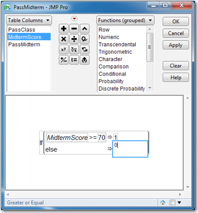
Select OK→OK.

First, let us use a traditional contingency table analysis to determine the odds ratio. Make sure that both PassClass and PassMidterm are classified as nominal variables. Right-click in the data grid of the column PassClass and select Column Info. Click the black triangle next to Modeling Type and select Nominal→OK. Do the same for PassMidterm.

Select Tables→Tabulate to open the Control Panel. It shows the general layout for a table. Drag PassClass into the Drop zone for columns and select Add Grouping Columns. Now that data have been added, the words Drop zone for rows will no longer be visible, but the Drop zone for rows will still be in the lower left panel of the table. See Figure 5.4.

Figure 5.4  Control Panel for Tabulate

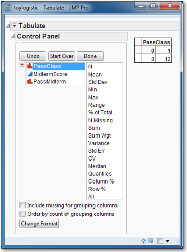
Drag PassMidterm to the panel immediately to the left of the 8 in the table. Select Add Grouping Columns. Click Done. A contingency table identical to Figure 5.5 will appear.

Figure 5.5  Contingency Table from toydataset.jmp

The probability of passing the class when you did not pass the midterm is

The probability of not passing the class when you did not pass the midterm is

(similar to row percentages). The odds of passing the class given that you have failed the midterm are

Similarly, we calculate the odds of passing the class given that you have passed the midterm as:

Of the students that did pass the midterm, the odds are the number of students that pass the class divided by the number of students that did not pass the class.

In the above paragraphs, we spoke only of odds. Now let us calculate an odds ratio. It is important to note that this can be done in two equivalent ways. Suppose we want to know the odds ratio of passing the class by comparing those who pass the midterm (PassMidterm=1 in the numerator) to those who fail the midterm (PassMidterm=0 in the denominator). The usual calculation leads to:

which has the following interpretation: the odds of passing the class are 8.33 times the odds of failing the course if you pass the midterm. This odds ratio can be converted into a probability. We know that P(Y=1)/P(Y=0)=8.33; and by definition, P(Y=1)+P(Y=0)=1. So solving two equations in two unknowns yields P(Y=0) = (1/(1+8.33)) = (1/9.33)= 0.1072 and P(Y=1) = 0.8928. As a quick check, observe that 0.8928/0.1072=8.33. Note that the log-odds are ln(8.33) = 2.120. Of course, the user doesn’t have to perform all these calculations by hand; JMP will do them automatically. When a logistic regression has been run, simply clicking the red triangle and selecting Odds Ratios will do the trick.

Equivalently, we could compare those who fail the midterm (PassMidterm=0 in the numerator) to those who pass the midterm (PassMidterm=1 in the denominator) and calculate:

.

which tells us that the odds of failing the class are 0.12 times the odds of passing the class for a student who passes the midterm. Since P(Y = 0) = 1 - π (the probability of failing the midterm) is in the numerator of this odds ratio, we must interpret it in terms of the event failing the midterm. It is easier to interpret the odds ratio when it is less than 1 by using the following transformation: (OR – 1)*100%. Compared to a person who passes the midterm, a person who fails the midterm is 12% as likely to pass the class; or equivalently, a person who fails the midterm is 88% less likely, (OR – 1)*100% = (0.12 – 1)*100%= -88%, to pass the class than someone who passed the midterm. Note that the log-odds are ln(0.12) = -2.12.

The relationships between probabilities, odds (ratios), and log-odds (ratios) are straightforward. An event with a small probability has small odds, and also has small log-odds. An event with a large probability has large odds and also large log-odds. Probabilities are always between zero and unity; odds are bounded below by zero but can be arbitrarily large; log-odds can be positive or negative and are not bounded, as shown in Figure 5.6. In particular, if the odds ratio is 1 (so the probability of either event is 0.50), then the log-odds equal zero. Suppose π = 0.55, so the odds ratio 0.55/0.45 = 1.222. Then we say that the event in the numerator is (1.222-1) = 22.2% more likely to occur than the event in the denominator.

Odds Ratios in Logistic Regression

Different software applications adopt different conventions for handling the expression of odds ratios in logistic regression. By default, JMP = uses the “log odds of 0/1” convention, which puts the 0 in the numerator and the 1 in the denominator. This is a consequence of the sort order of the columns, which we will address shortly.

Figure 5.6  Ranges of Probabilities, Odds, and Log-odds

To see the practical importance of this, rather than compute a table and perform the above calculations, we can simply run a logistic regression. It is important to make sure that PassClass is nominal and that PassMidterm is continuous. If PassMidterm is nominal, JMP will fit a different but mathematically equivalent model that will give different (but mathematically equivalent) results. The scope of the reason for this is beyond this book, but, in JMP, interested readers can consult Help→Books→Modeling and Multivariate Methods and refer to Appendix A.

If you have been following along with the book, both variables ought to be classified as nominal, so PassMidterm needs to be changed to continuous. Right-click in the column PassMidterm in the data grid and select Column Info. Click the black triangle next to Modeling Type and select Continuous, and then click OK.

Now that the dependent and independent variables are correctly classified as Nominal and Continuous, respectively, let’s run the logistic regression:

From the top menu, select Analyze→Fit Model. Select PassClass→Y. Select PassMidterm→Add. The Fit Model dialog box should now look like Figure 5.7. Click Run.

Figure 5.7  Fit Model Dialog Box

Figure 5.8 displays the logistic regression results.

Figure 5.8  Logistic Regression Results for toylogistic.jmp

Examine the parameter estimates in Figure 5.8. The intercept is 0.91629073, and the slope is -2.1202635. The slope gives the expected change in the logit for a one-unit change in the independent variable (i.e., the expected change on the log of the odds ratio). However, if we simply exponentiate the slope (i.e., compute ), then we get the 0/1 odds ratio.

There is no need for us to exponentiate the coefficient manually. JMP will do this for us:

Click the red triangle and click Odds Ratios. The Odds Ratios tables are added to the JMP output as shown in Figure 5.9.

Figure 5.9  Odds Ratios Tables Using the Nominal Independent Variable PassMidterm

Unit Odds Ratios refers to the expected change in the odds ratio for a one-unit change in the independent variable. Range Odds Ratios refers to the expected change in the odds ratio when the independent variable changes from its minimum to its maximum. Since the present independent variable is a binary 0-1 variable, these two definitions are the same. We get not only the odds ratio, but a confidence interval, too. Notice the right-skewed confidence interval; this is typical of confidence intervals for odds ratios.

To change from the default convention (log odds of 0/1, which puts the 0 in the numerator and the 1 in the denominator, in the data table), right-click to select the name of the PassClass column. Under Column Properties, select Value Ordering. Click on the value 1 and click Move Up as in Figure 5.10.

Figure 5.10  Changing the Value Order

Then, when you re-run the logistic regression, although the parameter estimates will not change, the odds ratios will change to reflect the fact that the 1 is now in the numerator and the 0 is in the denominator.

The independent variable is not limited to being only a nominal (or ordinal) dependent variable; it can be continuous. In particular, let’s examine the results using the actual score on the midterm, with MidtermScore as an independent variable:

Select Analyze→Fit Model. Select PassClass→Y and then select MidtermScore→Add. Click Run.

This time the intercept is 25.6018754, and the slope is -0.3637609. So we expect the log-odds to decrease by 0.3637609 for every additional point scored on the midterm, as shown in Figure 5.11.

Figure 5.11  Parameter Estimates

To view the effect on the odds ratio itself, as before click the red triangle and click Odds Ratios. Figure 5.12 displays the Odds Ratios tables.

Figure 5.12  Odds Ratios Tables Using the Continuous Independent Variable MidtermScore

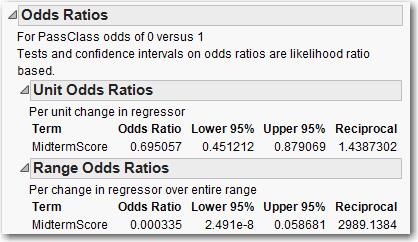
For a one-unit increase in the midterm score, the new odds ratio will be 69.51% of the old odds ratio. Or, equivalently, we expect to see a 30.5% reduction in the odds ratio (0.695057 – 1)*(100%=-30.5%). For example, suppose a hypothetical student has a midterm score of 75%. The student’s log odds of failing the class would be 25.6018754 – 0.3637609*75 = -1.680192. So the student’s odds of failing the class would be exp(-1.680192) = 0.1863382. That is, the student is much more likely to pass than fail. Converting odds to probabilities (0.1863328/(1+0.1863328) = 0.157066212786159), we see that the student’s probability of failing the class is 0.15707, and the probability of passing the class is 0.84293. Now, if the student’s score increased by one point to 76, then the log odds of failing the class would be 25.6018754 – 0.3637609*76 = -2.043953. Thus, the student’s odds of failing the class become exp(-2.043953)= 0.1295157. So, the probability of passing the class would rise to 0.885334, and the probability of failing the class would fall to 0.114666. With respect to the Unit Odds Ratio, which equals 0.695057, we see that a one-unit increase in the test score changes the odds ratio from 0.1863382 to 0.1295157. In accordance with the estimated coefficient for the logistic regression, the new odds ratio is 69.5% of the old odds ratio because 0.1295157/0.1863382 = 0.695057.

Finally, we can use the logistic regression to compute probabilities for each observation. As noted, the logistic regression will produce an estimated logit for each observation. These estimated logits can be used, in the obvious way, to compute probabilities for each observation. Consider a student whose midterm score is 70. The student’s estimated logit is 25.6018754 – 0.3637609(70) = 0.1386124. Since exp(0.1386129) = 1.148679 = p/(1-p), we can solve for p (the probability of failing) = 0.534597.

We can obtain the estimated logits and probabilities by clicking the red triangle on Normal Logistic Fit and selecting Save Probability Formula. Four columns will be added to the worksheet: Lin[0], Prob[0], Prob[1], and Most Likely PassClass. For each observation, these give the estimated logit, the probability of failing the class, and the probability of passing the class, respectively. Observe that the sixth student has a midterm score of 70. Look up this student’s estimated probability of failing (Prob[0]); it is very close to what we just calculated above. See Figure 5.13. The difference is that the computer carries 16 digits through its calculations, but we carried only six.

Figure 5.13  Verifying Calculation of Probability of Failing

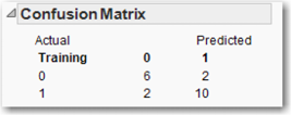
The fourth column (Most Likely PassClass) classifies the observation as either 1 or 0, depending upon whether the probability is greater than or less than 50%. We can observe how well our model classifies all the observations (using this cut-off point of 50%) by producing a confusion matrix: Click the red triangle and click Confusion matrix. Figure 5.14 displays the confusion matrix for our example. The rows of the confusion matrix are the actual classification (that is, whether PassClass is 0 or 1). The columns are the predicted classification from the model (that is, the predicted 0/1 values from that last fourth column using our logistic model and a cutpoint of .50). Correct classifications are along the main diagonal from upper left to lower right. We see that the model has classified 6 students as not passing the class, and actually they did not pass the class. The model also classifies 10 students as passing the class when they actually did. The values on the other diagonal, both equal to 2, are misclassifications. The results of the confusion matrix will be examined in more detail when we discuss model comparison in Chapter 9.

Figure 5.14  Confusion Matrix

Of course, before we can use the model, we have to check the model’s assumptions, etc. The first step is to verify the linearity of the logit. This can be done by plotting the estimated logit against PassClass. Select Graph→Scatterplot Matrix. Select Lin[0]→Y, columns. Select MidtermScore→X. Click OK. As shown in Figure 5.15, the linearity assumption appears to be perfectly satisfied.

Figure 5.15  Scatterplot of Lin[0] and MidtermScore

The analog to the ANOVA F-test for linear regression is found under the Whole Model Test, shown in Figure 5.16, in which the Full and Reduced models are compared. The null hypothesis for this test is that all the slope parameters are equal to zero. Since Prob>ChiSq is 0.0004, this null hypothesis is soundly rejected. For a discussion of other statistics found here, such as BIC and Entropy RSquare, see the JMP Help.

Figure 5.16  Whole Model Test for the Toylogistic Data Set

The next important part of model checking is the Lack of Fit test. See Figure 5.17. It compares the model actually fitted to the saturated model. The saturated model is a model generated by JMP that contains as many parameters as there are observations. So it fits the data very well. The null hypothesis for this test is that there is no difference between the estimated model and the saturated model. If this hypothesis is rejected, then more variables (such as cross-product or squared terms) need to be added to the model. In the present case, as can be seen, Prob>ChiSq=0.7032. We can therefore conclude that we do not need to add more terms to the model.

Figure 5.17  Lack of Fit Test for Current Model

A Logistic Regression Statistical Study

Let’s turn now to a more realistic data set with several independent variables. During this discussion, we will also present briefly some of the issues that should be addressed and some of the thought processes during a statistical study.

Cellphone companies are very interested in determining which customers might switch to another company; this is called “churning.” Predicting which customers might be about to churn enables the company to make special offers to these customers, possibly stemming their defection. Churn.jmp contains data on 3333 cellphone customers, including the variable Churn (0 means the customer stayed with the company and 1 means the customer left the company).

Before we can begin constructing a model for customer churn, we need to discuss model building for logistic regression. Statistics and econometrics texts devote entire chapters to this concept. In several pages, we can only sketch the broad outline. The first thing to do is make sure that the data are loaded correctly. Observe that Churn is classified as Continuous; be sure to change it to Nominal. One way is to right-click in the Churn column in the data table, select Column Info, and under Modeling Type, click Nominal. Another way is to look at the list of variables on the left side of the data table, find Churn, click the blue triangle (which denotes a continuous variable), and change it to Nominal (the blue triangle then becomes a red histogram). Make sure that all binary variables are classified as Nominal. This includes Intl_Plan, VMail_Plan, E_VMAIL_PLAN, and D_VMAIL_PLAN. Should Area_Code be classified as Continuous or Nominal? (Nominal is the correct answer!) CustServ_Call, the number of calls to customer service, could be treated as either continuous or nominal/ordinal; we treat it as continuous.

When building a linear regression model and the number of variables is not so large that this cannot be done manually, one place to begin is by examining histograms and scatterplots of the continuous variables, and crosstabs of the categorical variables as discussed in Chapter 3. Another very useful device as discussed in Chapter 3 is the scatterplot/correlation matrix, which can, at a glance, suggest potentially useful independent variables that are correlated with the dependent variable. The scatterplot/correlation matrix approach cannot be used with logistic regression, which is nonlinear, but a method similar in spirit can be applied.

We are now faced with a similar situation that was discussed in Chapter 4. Our goal is to build a model that follows the principle of parsimony—that is, a model that explains as much as possible of the variation in Y and uses as few significant independent variables as possible. However, now with multiple logistic regression, we are in a nonlinear situation. We have four approaches that we could take. We briefly list and discuss each of these approaches and some of their advantages and disadvantages:

■ Include all the variables. In this approach you just input all the independent variables into the model. An obvious advantage of this approach is that it is fast and easy. However, depending on the data set, most likely several independent variables will be insignificantly related to the dependent variable. Including variables that are not significant can cause severe problems—weakening the interpretation of the coefficients and lessening the prediction accuracy of the model. This approach definitely does not follow the principle of parsimony, and it can cause numerical problems for the nonlinear solver that may lead to a failure to obtain an answer.

■ Bivariate method. In this approach, you search for independent variables that may have predictive value for the dependent variable by running a series of bivariate logistic regressions; i.e., we run a logistic regression for each of the independent variables, searching for “significant” relationships. A major advantage of this approach is that it is the one most agreed upon by statisticians (Hosmer and Lemeshow, 2001). On the other hand, this approach is not automated, is very tedious, and is limited by the analyst’s ability to run the regressions. That is, it is not practical with very large data sets. Further, it misses interaction terms, which, as we shall see, can be very important.

■ Stepwise. In this approach, you would use the Fit Model platform, change the Personality to Stepwise and Direction to Mixed. The Mixed option is like Forward Stepwise, but variables can be dropped after they have been added. An advantage of this approach is that it is automated; so, it is fast and easy. The disadvantage of stepwise is that it could lead to possible interpretation and prediction errors depending on the data set. However, using the Mixed option, as opposed to the Forward or Backward Direction option, tends to lessen the magnitude and likelihood of these problems.

■ Decision Trees. A Decision Tree is a data mining technique that can be used for variable selection and will be discussed in Chapter 8. The advantage of using the decision tree technique is that it is automated, fast, and easy to run. Further, it is a popular variable reduction approach taken by many data mining analysts (Pollack, 2008). However, somewhat like the stepwise approach, the decision tree approach could lead to some statistical issues. In this case, significant variables identified by a decision tree are very sample-dependent. These issues will be discussed further in Chapter 8.

No one approach is a clear cut winner. Nevertheless, we do not recommend using the “Include all the variables” approach. If the data set is too large and/or you do not have the time, we recommend that you run both the stepwise and decision trees models and compare the results. The data set churn.jmp is not too large, so we will apply the bivariate approach.

It is traditional to choose α = 0.05. But in this preliminary stage, we adopt a more lax standard, α = 0.25. The reason for this is that we want to include, if possible, a group of variables that individually are not significant but together are significant. Having identified an appropriate set of candidate variables, run a logistic regression including all of them. Compare the coefficient estimates from the multiple logistic regression with the estimates from the bivariate logistic regressions. Look for coefficients that have changed in sign or have dramatically changed in magnitude, as well as changes in significance. Such changes indicate the inadequacy of the simple bivariate models, and confirm the necessity of adding more variables to the model.

Three important ways to improve a model are as follows:

■ If the logit appears to be nonlinear when plotted against some continuous variable, one resolution is to convert the continuous variable to a few dummies, say three, that cut the variable at its 25^th, 50^th, and 75^th percentiles.

■ If a histogram shows that a continuous variable has an excess of observations at zero (which can lead to nonlinearity in the logit), add a dummy variable that equals one if the continuous variable is zero and equals zero otherwise.

■ Finally, a seemingly numeric variable that is actually discrete can be broken up into a handful of dummy variables (e.g., ZIP codes).

Before we can begin modeling, we must first explore the data. With our churn data set, creating and examining the histograms of the continuous variables reveals nothing much of interest, except VMail_Message, which has an excess of zeros. (See the second point in the previous paragraph.) Figure 5.18 shows plots for Intl_Calls and VMail_Message. To produce such plots, select Analyze→Distribution, click Intl_Calls, and then Y, Columns and OK. To add the Normal Quantile Plot, click the red arrow next to Intl_Calls and select Normal Quantile Plot. Here it is obvious that Intl_Calls is skewed right. We note that a logarithmic transformation of this variable might be in order, but we will not pursue the idea.

Figure 5.18  Distribution of Intl_Calls and VMail_Message

A correlation matrix of the continuous variables (select Graph→Scatterplot Matrix and put the desired variables in Y, Columns) turns up a curious pattern. Day_Charge and Day_Mins, Eve_Charge and Eve_Mins, Night_Charge and Night_Mins, and Intl_Charge and Intl_Mins all are perfectly correlated. The charge is obviously a linear function of the number of minutes. Therefore, we can drop the Charge variables from our analysis. (We could also drop the “Mins” variables instead; it doesn’t matter which one we drop.) If our data set had a very large number of variables, the scatterplot matrix would be too big to comprehend. In such a situation, we would choose groups of variables for which to make scatterplot matrices, and examine those.

A scatterplot matrix for the four binary variables turns up an interesting association. E_VMAIL_PLAN and D_VMAIL_PLAN are perfectly correlated; both have common 1s and where the former has -1, the latter has zero. It would be a mistake to include both of these variables in the same regression (try it and see what happens). Let’s delete E_VMAIL_PLAN from the data set and also delete VMail_Plan because it agrees perfectly with E_VMAIL_PLAN: When the former has a “no,” the latter has a “-1,” and similarly for “yes” and “+1.”

Phone is more or less unique to each observation. (We ignore the possibility that two phone numbers are the same but have different area codes.) Therefore, it should not be included in the analysis. So, we will drop Phone from the analysis.

A scatterplot matrix between the remaining continuous and binary variables turns up a curious pattern. D_VMAIL_PLAN and VMailMessage have a correlation of 0.96. They have zeros in common, and where the former has 1s, the latter has numbers. (See again point two in the above paragraph. We won’t have to create a dummy variable to solve the problem because D_VMAIL_PLAN will do the job nicely.)

To summarize, we have dropped 7 of the original 23 variables from the data set (Phone, Day_Charge, Eve_Charge, Night_Charge, Intl_Charge, E_VMAIL_PLAN, and VMail_Plan). So there are now 16 variables left, one of which is the dependent variable, Churn. We have 15 possible independent variables to consider.

Next comes the time-consuming task of running several bivariate (two variables, one dependent and one independent) analyses, some of which will be logistic regressions (when the independent variable is continuous) and some of which will be contingency tables (when the independent variable is categorical). In total, we have 15 bivariate analyses to run. What about Area Code? JMP reads it as a continuous variable, but it’s really nominal, so make sure to change it from continuous to nominal. Similarly, make sure that D_VMAIL_PLAN is set as a nominal variable, not continuous.

Do not try to keep track of the results in your head, or by referring to the 15 bivariate analyses that would fill your computer screen. Make a list of all 15 variables that need to be tested, and write down the test result (e.g., the relevant p-value) and your conclusion (e.g., “include” or “exclude”). This not only prevents simple errors; it is a useful record of your work should you have to come back to it later. There are few things more pointless than conducting an analysis that concludes with a 13-variable logistic regression, only to have some reason to rerun the analysis and now wind up with a 12-variable logistic regression. Unless you have documented your work, you will have no idea why the discrepancy exists or which is the correct regression.

Below we briefly show how to conduct both types of bivariate analyses, one for a nominal independent variable and one for a continuous independent variable. We leave the other 14 to the reader.

Make a contingency table of Churn versus State: Select Analyze→Fit Y by X, click Churn (which is nominal) and then click Y, Response, click State and then click X, Factor; and click OK. At the bottom of the table of results are the Likelihood Ratio and Pearson tests, both of which test the null hypothesis that State does not affect Churn, and both of which reject the null. The conclusion is that the variable State matters. On the other hand, perform a logistic regression of Churn on VMail_Message: select Analyze→Fit Y by X, click Churn, click Y, Response, and click VMail_Message and click X, Factor; and click OK. Under “Whole Model Test” that Prob>ChiSq, the p-value is less than 0.0001, so we conclude that VMail_message affects Churn. Remember that for all these tests, we are setting α (probability of Type I error) = 0.25.

In the end, we have 10 candidate variables for possible inclusion in our multiple logistic regression model:

State	Intl_Plan	D_VMAIL_PLAN
VMail_Message	Day_Mins	Eve_Mins
Night_Mins	Intl_Mins	Intl_Calls
CustServ_Call

Remember that the first three of these variables (the first row) should be set to nominal, and the rest to continuous. (Of course, leave the dependent variable Churn as nominal!)

Let’s run our initial multiple logistic regression with Churn as the dependent variable and the above 10 variables as independent variables:

Select Analyze→Fit Model→Churn→Y. Select the above 10 variables (to select variables that are not consecutive, click on each variable while holding down the Ctrl key), and click Add. Check the box next to Keep dialog open. Click Run.

The Whole Model Test lets us know that our included variables have an effect on the Churn and a p-value less than .0001, as shown in Figure 5.19.

Figure 5.19  Whole Model Test and Lack of Fit for the Churn Data Set

The lack-of-fit test tells us that we have done a good job explaining Churn. From the Lack of Fit, we see that –LogLikelihood for the Full model is 1037.4471. Now, linear regression minimizes the sum of squared residuals. So when you compare two linear regressions, the preferred one has the smaller sum of squared residuals. In the same way, the nonlinear optimization of the logistic regression minimizes the –LogLikelihood (which is equivalent to maximizing the LogLikelihood). So the model with the smaller –LogLikelihood is preferred to a model with a larger –LogLikelihood.

Examining the p-values of the independent variables in the Parameter Estimates, we find that a variable for which Prob>ChiSq is less than 0.05 is said to be significant. Otherwise, it is said to be insignificant, similar to what is practiced in linear regression. The regression output gives two sets of tests, one for the “Parameter Estimates” and another for “Effect Likelihood Ratio Tests.” We shall focus on the latter. To see why, consider the State variable, which is really not one variable but many dummy variables. We are not so much interested in whether any particular state is significant or not (which is what the Parameter Estimates tell us) but whether, overall, the collection of state dummy variables is significant. This is what the Effect Likelihood Ratio Tests tells us; the effect of all the state dummies is significant with a “Prob>ChiSq” of 0.0010. True, many of the State dummies are insignificant, but overall State is significant; we will keep this variable as it is. It may prove worthwhile to reduce the number of state dummies into a handful of significant states and small clusters of “other” states that are not significant, but we will not pursue this line of inquiry here.

We can see that all the variables in the model are significant. We may be able to derive some new variables that help improve the model. We will provide two examples of deriving new variables—(1) Converting a continuous variable into discrete variables; (2) Producing interaction variables.

Let us try to break up a continuous variable into a handful of discrete variables. An obvious candidate is CustServ_Call. Look at its distribution in Figure 5.20. Select Analyze→Distribution, select CustServ_Call→Y, Columns, and click OK. Click the red arrow next to CustServ_Call and uncheck Outlier Box Plot. Then choose Histogram Options→Show Counts.

Figure 5.20  Histogram of CustServ_Call

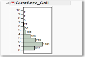
Let’s create a new nominal variable called CustServ, so that all the counts for 5 and greater are collapsed into a single cell:

Select Cols→New Columns. For column name type CustServ, for Modeling Type change it to Nominal and then click the drop-down arrow for Column Properties and click Formula. In the Formula dialog box, select Conditional→If. Then, in the top expr, click CustServ_Call and type <=4. In the top then clause, click CustServ_Call. For the else clause, type 5. See Figure 5.21. Click OK and click OK.

Figure 5.21  Creating the CustServ Variable

Now drop the CustServ_Call variable from the Logistic Regression and add the new CustServ nominal variable, which is equivalent to adding some dummy variables. Our new value of -LogLikelihood is 970.6171, which constitutes a very substantial improvement in the model.

Another possible important way to improve a model is to introduce interactions terms, that is, the product of two or more variables. Best practice would be to consult with subject-matter experts and seek their advice. Some thought is necessary to determine meaningful interactions, but it can pay off in substantially improved models. Thinking about what might make a cell phone customer want to switch to another carrier, we have all heard a friend complain about being charged an outrageous amount for making an international call. Based on this observation, we could conjecture that customers who make international calls and who are not on the international calling plan might be more irritated and more likely to churn. A quick bivariate analysis shows that there are more than a few such persons in the data set. Select Tables→Tabulate, and drag Intl_Plan to Drop zone for columns. Drag Intl_Calls to Drop zone for rows. Click Add Grouping Columns. Observe that almost all customers make international calls, but most of them are not on the international plan (which gives cheaper rates for international calls). For example, for the customers who made no international call, all 18 of them were not on the international calling plan. For the customers who made 8 international calls, 106 were not on the international calling plan, and only 10 of them were. There is quite the potential for irritated customers here! This is confirmed by examining the output from the previous logistic regression. The parameter estimate for “Intl_Plan[no]” is positive and significant. This means that when a customer does not have an international plan, the probability is that the churn increases.

Customers who make international calls and don’t get the cheap rates are perhaps more likely to churn than customers who make international calls and get cheap rates. Hence, the interaction term Int_Plan*Intl_Mins might be important. To create this interaction term, we have to create a new dummy variable for Intl_Plan, because the present variable is not numeric and cannot be multiplied by Intl_Mins:

First, click on the Intl_Plan column in the data table to select it. Then select Cols→Recode. Under New Value, where it has No, type 0 and right below that where it has Yes, type 1. From the In Place drop-down menu, select New Column and click OK. The new variable Intl_Plan2 is created. However, it is still nominal. Right-click on this column and under Column Info, change the Data Type to Numeric and the Modeling Type to Continuous. Click OK. (This variable has to be continuous so that we can use it in the interaction term, which is created by multiplication; nominal variables cannot be multiplied.)

To create the interaction term:

Select Cols→New Column and call the new variable IntlPlanMins. Under Column Properties, click Formula. Click Intl_Plan2, click on the times sign (x) in the middle of the dialog box, click Intl_Mins and click OK. Click OK again.

Now add the variable IntlPlanMins as the 11^th independent variable in multiple logistic regression that includes CustServ and run it. The variable IntlPlanMins is significant, and the –LogLikelihood has dropped to 947.1450, as shown in Figure 5.22. This is a substantial drop for adding one variable. Doubtless other useful interaction terms could be added to this model, but we will not further pursue this line of inquiry.

Figure 5.22  Logistic Regression Results with Interaction Term Added

Now that we have built an acceptable model, it is time to validate the model. We have already checked the Lack of Fit, but now we have to check linearity of the logit. From the red arrow, click Save Probability Formula, which adds four variables to the data set: Lin[0] (which is the logit), Prob[0], Prob[1], and the predicted value of Churn, Most Likely Churn. Now we have to plot the logit against each of the continuous independent variables. The categorical independent variables do not offer much opportunity to reveal nonlinearity (plot some and see this for yourself). All the relationships of the continuous variables can be quickly viewed by generating a scatterplot matrix and then clicking the red triangle and Fit Line. Nearly all the red fitted lines are horizontal or near horizontal. For all of the logit vs. independent variable plots, there is no evidence of nonlinearity.

We can also see how well our model is predicting by examining the confusion matrix, which is shown in Figure 5.23.

Figure 5.23  Confusion Matrix

The actual number of churners in the data set is 326+157 = 483. The model predicted a total of 258 (=101+157) churners. The number of bad predictions made by the model is 326+101 = 427, which indicates that 326 that were predicted not to churn actually did churn, and 101 that were predicted to churn did not churn. Further, observe in the Prob[1] column of the data table that we have the probability that any customer will churn. Right-click on this column and select Sort. This will sort all the variables in the data set according to the probability of churning. Scroll to the top of the data set. Look at the Churn column. It has mostly ones and some zeros here at the top, where the probabilities are all above 0.85. Scroll all the way to the bottom and see that the probabilities now are all below 0.01, and the values of Churn are all zero. We really have modeled the probability of churning.

Now that we have built a model for predicting churn, how might we use it? We could take the next month’s data (when we do not yet know who has churned) and predict who is likely to churn. Then these customers can be offered special deals to keep them with the company, so that they do not churn.

References

Hosmer, D. W., and S. Lemeshow. (2001). Applied Logistic Regression. 2nd ed. New York: John Wiley & Sons.

Pollack, R. (2008). “Data Mining: Common Definitions, Applications, and Misunderstandings.” Data Mining Methods and Applications (Discrete Mathematics & Its Applications). Lawrence, K. D., S. Kudyba, and R. K. Klimberg (Eds.). Boca Raton, FL: Auerbach Publications.

Exercises 

1. Consider the logistic regression for the toy data set, where π is the probability of passing the class:

Consider two students, one who scores 67% on the midterm and one who scores 73% on the midterm. What are the odds that each fails the class? What is the probability that each fails the class?

2. Consider the first logistic regression for the Churn data set, the one with 10 independent variables. Consider two customers, one with an international plan and one without. What are the odds that each churns? What is the probability that each churns?

3. We have already found that the interaction term IntlPlanMins significantly improves the model. Find another interaction term that does so.

4. Without deriving new variables such as CustServ or creating interaction terms such as IntlPlanMins, use a stepwise method to select variables for the Churn data set. Compare your results to the bivariate method used in the chapter; pay particular attention to the fit of the model and the confusion matrix.

5. Use the Freshmen1.jmp data set and build a logistic regression model to predict whether a student returns. Perhaps the continuous variables Miles from Home and Part Time Work Hours do not seem to have an effect. See whether turning them into discrete variables makes a difference. (E.g., turn Miles from Home into some dummy variables, 0‒20 miles, 21‒100 miles, more than 100 miles.)