
Chapter 16: Multivariate GARCH Models
A Bivariate Example Using Two Quotations for Danish Stocks
Using the CCC Parameterization
Using the DCC Parameterization
Using the BEKK Parameterization
Using the CCC Bivariate Combination of Univariate TGARCH Models
Introduction
In this chapter you will see how the VARMAX procedure is applied to estimate the parameters of GARCH models for multivariate time series. The theoretical specification of the model follows the outline for the univariate case in Chapter 15. The extension from univariate to multivariate time series is presented in the first section. Procedure syntax for estimation and checking for model fit is demonstrated by the examples in the remaining sections of this chapter.
Multivariate GARCH Models
In the literature, several ideas for multivariate GARCH models exist: BEKK, CCC, and DCC. The BEKK parameterization is a straightforward extension of the basic standard GARCH formulation to a multivariate expression using matrices. The CCC and the DCC parameterizations are ways to combine univariate GARCH models to cover the multivariate situation by the introduction of only a few extra parameters.
The CCC and the DCC parameterizations allow for alternative parameterizations of the GARCH models for the individual univariate series, models such as PGARCH and TGARCH. (See Chapter 15.)
The CCC Parameterization
The CCC (Constant Conditional Correlation) parameterization simply combines GARCH models for the individual time series, using a constant correlation between each pair of series. This gives a rather simple model: Just a single parameter is applied to model the dependence between two variance processes. The two other methods introduce many more parameters, which can lead to numerical instabilities.
The correlations among the k series are combined into a k ×k matrix, denoted S. The (i,j) entry is denoted sij, i, j = 1, . . . , k. The GARCH models for the individual series define conditional variances for each series separately. Let hiit denote the conditional variance for the ith series in accordance with the notation used in Chapter 15. However, use an extra i in the subscript to catch up with the matrix notation. The volatility model for the conditional variances hiit can be a usual GARCH model, but the alternative versions, such as QGACH and TGARCH, are also allowed.
The dependence among the series is then described by the covariance, hijt, conditioned on the past values. The conditional covariance is now defined as follows:
In this formula, the constant correlation is simply multiplied by the two conditional standard deviations in order to define the conditional covariance.
In this parameterization, only one parameter is introduced for each pair of series, compared to univariate GARCH models for the separate series when the volatility structures are assumed to be independent. For the bivariate case, a CCC-GARCH(1,1) model includes three parameters for each univariate GARCH model and a single extra parameter, the correlation between the series. In the bivariate case, this gives seven parameters.
An intuitive way to build a CCC model is to estimate GARCH models for each individual series—that is, to estimate the parameters in the k individual models:
The estimation of a CCC model can be performed by k separate applications of PROC VARMAX for each of the k series. After that, the correlations sij in the matrix S can be estimated by the empirical correlation:
In PROC VARMAX, this method is available by a special option, but the default method is simultaneous estimation of all parameters using maximum likelihood estimation.
The DCC Parameterization
The DCC specification of a multivariate GARCH model introduces a Dynamic Conditional Correlation, as the name indicates. This dynamic correlation is defined by considering the correlation sijt at time t in the CCC parameterization as a time series in its own right.
The volatility model for the conditional variances hiit could be in the CCC parameterization a usual GARCH model but also QGACH, TGARCH, and the other variations are allowed. The conditional covariance hijt at time t between the ith and the jth series conditioned upon past values is defined as a weighted average of previous products of the time series values and the previous conditional covariance. This idea mirrors the definition of ARMA(1,1) and GARCH(1,1) models.
The conditional correlation sijt is defined as follows:
In this expression, the parameter sij (without the sub index t) is the unconditional correlation. The idea is that the correlation between the two series also includes some volatility. This means that the correlation could be high in times of, say, crises in the market where the factors εit are large. But the correlation is less pronounced in stable time periods with values of εit close to 0.
The DCC-GARCH(1,1) model for a bivariate series includes three extra parameters, α, β, and s12, in the model for the combination of the GARCH(1,1) models for each series. Because each individual model contains three parameters, this gives a total of nine parameters, which is two more than for the CCC parameterization.
The parameter sij for the unconditional correlation can be initially estimated by the following:
This value can also be fixed as in the CCC model by an option in PROC VARMAX. If the value is fixed, then the numerical estimation of the remaining parameters is simplified because one less parameter has to be estimated.
The BEKK Parameterization
The acronym BEKK is derived from the names of four authors who introduced this particular parameterization. The BEKK representation is a straightforward generalization of univariate GARCH models to the multivariate situation by replacing all scalar parameters, numbers, and products of numbers by matrices using matrix multiplication.
The BEKK parameterization for a multivariate time series, yt, the covariance matrix of Ht at time t is conditioned on past values yt−i of the multivariate series yt and past covariance matrices Ht−i is given by the following:
The matrix C is a symmetric matrix. The matrix H is assumed to be positive definite. In the bivariate case, the symmetric matrix C includes 3 parameters; the two 2-by-2 matrices A and G each include 4 parameters. The model in total includes 11 parameters for p = q = 1.
It is illustrative to write the BEKK parameterization of a bivariate GARCH(1,1) model in equation form. Doing so is especially important because these equations show why the coefficients in PROC VARMAX are defined in a different way from the similar equations in Chapter 15. In short, the coefficients in this chapter are more intuitive in the univariate situation than their square roots, which are printed as estimates by PROC VARMAX. However, in multivariate contexts, the default BEKK parameterization used by PROC VARMAX is natural. The option FORM=CCC, which was applied in Chapter 15, turns the parameterization into the form used in Chapter 15.
The conditional variances and covariances in a BEKK parameterization of a bivariate GARCH(1,1) model, in equation form, have the following form:
In the univariate case, this form reduces to the following:
where the coefficients are squared compared to the usual GARCH parameterization.
The number of parameters in the BEKK parameterization even for a two-dimensional time series is large, and the parameter estimates are imprecise unless the time series are very long. The example in this chapter is unsuitable for illustrating the BEKK parameterization because it consists of only T = 248 observations.
A Bivariate Example Using Two Quotations for Danish Stocks
In this section, the example of quotations of a Danish bank discussed in Chapter 15 is extended with another quotation series. The second series is a series of quotations of a Danish biotechnology company. The variable PERCENTAGE_CHANGE_BIOTECH denotes the series of differences expressed as percentages.
The two series are plotted by Program16.1.
Program 16.1: Plotting the Relative Day-to-Day Changes of the Quotation of Two Danish Stocks
PROC SGPLOT DATA=SASMTS.QUOTES;
SERIES X=I Y=PERCENTAGE_CHANGE_BANK;
SCATTER X=I Y=PERCENTAGE_CHANGE_BIOTECH;
RUN;
The two series have a similar volatility structure. See Figure 16.1. At least some periods show low variation for both series. The periods of higher volatility are more difficult to describe, but they are also simultaneous to some extent.
Figure 16.1: Plots of the Relative Day-to-Day Changes of the Quotation of Two Danish Stocks

Using the CCC Parameterization
In Program 16.2, the bivariate GARCH(1,1) model with the CCC parameterization is fitted. This particular parameterization is used first because it includes only one parameter for the covariance between the two series.
Program 16.2: Estimating a CCC Parameterization for a Bivariate Series of Quotations
PROC VARMAX DATA=SASMTS.QUOTES;
MODEL PERCENTAGE_CHANGE_BANK PERCENTAGE_CHANGE_BIOTECH/NOINT;
GARCH Q=1 P=1 FORM=CCC OUTHT=OUTHT;
RUN;
The resulting parameters are presented in Output 16.1.
Output 16.1: Estimated Parameters in the CCC-GARCH(1,1) Model
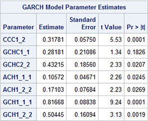
In this CCC-GARCH(1,1) model, two univariate GARCH(1,1) models are estimated: one for each separate series. For the estimated parameters, these models are written as follows:
for the bank series, and
for the biotech series.
The conditional variances h1t and h2t for these series are then combined by a constant correlation, s12, using the following formula:
The constant correlation is estimated by .32. This is denoted CCC_1_2 in Output 16.1. This estimated value is almost equal to the usual correlation coefficient between the two series, which is estimated as .34 by PROC CORR.
The correlation coefficient can be fixed by the option CORRCONSTANT=EXPECT to the GARCH statement. In this case, the GARCH parameters are estimated by nearly the same numbers as in Output 16.1. The correlation is printed, along with the GARCH parameters, in Output 16.2.
Output 16.2: Estimated Parameters with a Restricted Correlation

Using the DCC Parameterization
In this subsection, the estimated CCC parameterization is extended to the DCC parameterization by allowing the correlation function to be time varying, because the correlation is also considered as a time series having its own time series model.
A first estimation is performed by Program 16.3.
Program 16.3: Estimating a DCC Parameterization for a Bivariate Series of Quotations
PROC VARMAX DATA=SASMTS.QUOTES;
MODEL PERCENTAGE_CHANGE_BANK PERCENTAGE_CHANGE_BIOTECH/NOINT;
GARCH Q=1 P=1 FORM=DCC OUTHT=OUTHT;
RUN;
The results (Output 16.3) are, however, somehow disappointing. All estimated parameters are close to zero, and most of the reported standard deviations are missing or printed as zero. This result is due to over-parameterization as the estimation algorithm has run into problems. In short, the problem is that the likelihood function is much less informative to GARCH parameters than to the linear parameters considered in Chapters 1–12.
Output 16.3: Parameters in the DCC GARCH(1,1) Model as Estimated by Program 16.3

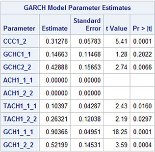
A natural remedy is to include the results from the fitted CCC parameterization in the previous subsection as starting values for the iterations in the estimation algorithm. This is possible with the use of the INITIAL statement in Program 16.4. In this initial statement, the parameters are denoted by replacing the numbers for lags and series in Output 16.3 by numbers in brackets. For instance, GCH1_1_1 in Output 16.3 is written as GCH(1,1,1) in Program 16.4.
Program 16.4: Estimating a DCC Parameterization Using Initial Values for the Parameters
PROC VARMAX DATA=SASMTS.QUOTES;
MODEL PERCENTAGE_CHANGE_BANK PERCENTAGE_CHANGE_BIOTECH/NOINT;
GARCH Q=1 P=1 FORM=DCC OUTHT=OUTHT;
INITIAL GCHC(1,1)=0.28,GCHC(2,2)=0.43,ACH(1,1,1)=0.11,
GCH(1,1,1)=0.82,ACH(1,2,2)=0.17,GCH(1,2,2)=0.50;
RUN;
The results (Output 16.4) are in most respects close to the results of the CCC parameterization that was presented on Output.16.2. But some of the standard deviations of the estimated parameters are not written to the output. This is a clear indication that the fitted model is too ambitious for the data at hand.
Output 16.4: Estimated DCC_GARCH(1,1) Parameters

If a further statement is included in Program 16.4, then the hypothesis that the two extra parameters α and β both equal zero is tested:
TEST DCCA=0,DCCB=0;
This hypothesis is clearly accepted. See Output 16.5.
Output 16.5: Simultaneous Test for the Parameters α and β, Both Being 0

When this hypothesis of α and β both being equal to zero is accepted, the DCC model reduces to the CCC model. In this way, it might be concluded that the dubious estimation results were caused by overfitting—that is, by inclusion of the superfluous parameters α and β. The extension from a CCC to a DCC parameterization seems to be superfluous in this example.
Using the BEKK Parameterization
The default parameterization of multivariate GARCH models in PROC VARMAX is the BEKK parameterization. This parameterization includes many parameters that, in light of the results by fitting the parameters of the DCC model, are expected to lead to some numerical problems for this data example.
In Program 16.5, all default settings are applied. Note that the FORM option is unnecessary in this application because BEKK is the default parameterization.
Program 16.5: Estimating the BEKK Parameterization in the Bivariate Case
PROC VARMAX DATA=SASMTS.QUOTES;
MODEL PERCENTAGE_CHANGE_BANK PERCENTAGE_CHANGE_BIOTECH/NOINT;
GARCH Q=1 P=1;
RUN;
One conclusion from the estimation of the DCC parameterization was that the covariance between the two series was constant. The fit of the CCC parameterization was as good as the DCC parameterization because the two extra parameters that make the covariance time varying were insignificant.
It is not possible to reduce the BEKK parameterization to a strict CCC parameterization with a constant correlation between the two series by restricting certain parameters to zero. This is because the formula for the time-varying covariance includes some of the ARCH/GARCH parameters even for the individual univariate ARCH/GARCH models.
The off-diagonal entries in the A and G matrices can be fixed as 0 by the RESTRICT statement:
RESTRICT ACH(1,1,2)=0,ACH(1,2,1)=0,GCH(1,1,2)=0,GCH(1,2,1)=0;
The estimation results are, however, not promising, and it is concluded that the number of observations T = 248 is too small to estimate a reasonable BEKK parameterization. The CCC parameterization fits the covariance structure of the series well, and it includes fewer parameters.
Using the CCC Bivariate Combination of Univariate TGARCH Models
It is possible to apply other parameterizations of the univariate GARCH models when they are combined into multivariate models by the CCC or the DCC parameterization.
In Program 16.6, univariate TGARCH models are applied to both series of stock quotations because this parameterization worked well in Chapter 15. They are combined by a CCC parameterization. The FORM option to the GARCH statement tells how to combine the univariate models into a multivariate model. The SUBFORM option determines the parameterization for the univariate series. Note that the same parameterization has to be applied for every univariate series. The default is SUBFORM=BEKK.
In the application of the TGARCH models for the univariate series in Program 16.6, the α parameters are restricted to zero, because this parameter was insignificant in the application in Chapter 15.
Program 16.6: Estimation of the CCC Bivariate Combination of Univariate TGARCH Models
PROC VARMAX DATA=SASMTS.QUOTES;
MODEL PERCENTAGE_CHANGE_BANK PERCENTAGE_CHANGE_BIOTECH/NOINT;
GARCH Q=1 P=1 FORM=CCC SUBFORM=TGARCH OUTHT=CONDITIONAL;
RESTRICT ACH(1,1,1)=0,ACH(1,2,2)=0;
RUN;
The two restrictions on the α parameters are both accepted by the Lagrange multiplier tests. See Output 16.6.
Output 16.6: Test for Restrictions in the TGARCH-CCC Model

The remaining parameters are all significant. See Output 16.7.
Output 16.7 Estimated Parameters for the TGARCH-CCC Model
The correlation is constant in this CCC parameterization; the value is the CCC1_2 parameter .32 in Output 16.7.
Conclusion
PROC VARMAX is useful for estimation in multivariate time series models. It includes many variations of the GARCH model for multivariate time series.
The usefulness of PROC VARMAX is demonstrated in this chapter for a bivariate series of daily quotations of a Danish bank and a Danish biotech firm. In the example, a multivariate GARCH model is formulated by combing marginal univariate GARCH models for the two series in question with a constant covariance. Moreover, alternative versions of the marginal univariate GARCH models are supported. In the particular example, TGACH models are applied.