chapter four

using the data builder

The Data Builder is the SAS Visual Analytics application that lets you extract data from various sources, prepare data, and load data sets into the SAS LASR Analytic Server or other locations. If you recall from previous chapters, the LASR Analytic Server is where your data is placed before you can use it in the report building sections. Using the Data Builder, you have more flexibility with preparing and importing your data into the LASR Analytic Server. The Data Builder can also be used to create staging tables or load tables into the Hadoop Distributed File System (HDFS).

With the Data Builder, you can build queries around the data and then you can run those queries to manipulate and move the data to output locations. Data can be accessed through local files, databases, SAS data sets, and so on. While building your query, you have the option to perform minor data manipulation such as adding new data items, summarizing data, and even joining with other tables. The Data Builder does this through a user interface that is building SQL code in the background.

When SAS Visual Analytics moved from version 7.3 to 8.1, there was an overhaul to the Data Builder in regards to the interface (switch to HTML5) and functionality. This chapter focuses on the main aspects of the Data Builder and the capabilities of 7.3, Chapter 13 takes you through the 8.1 version and all of the updates that come with it.

Using the Data Builder

So why should you use the Data Builder instead of just importing the whole data set? For this, you must remember that LASR Analytic Server works on temporary memory. Therefore, any conditions, simple calculations, groupings, and so on, are just place holders. The real data is computed each time you interact with the data set. By doing some initial data prep in the Data Builder, you can polish your data set and have it ready before it even goes into the LASR Analytic Server.

The Data Builder should also be considered when you are trying to work with multiple data sets or append data sets in the LASR Analytic Server. There is access to tables in the LASR Analytic Server, and you can also import data from local files, servers, databases, and social media. With tables already in the LASR Analytic Server, there is functionality in the Data Builder to construct a query that appends to that table every time the query is run. When you want to join tables, queries can bring in multiple tables so that you can connect them as needed through a user interface or SQL code. You can even create an entire star schema if needed.

Creating a data query

A data query is your means to create a new table from a data source and then load it into a source. At its roots, a data query is a SAS program that connects you to your sources so that you can pull data from them. Then, the query performs everything necessary behind the scenes so that you can load into the LASR Analytic Server, send the query to HDFS, or create a staging table. In the Data Builder, queries also must be saved before you can use them. Once you save a query, you can then use it in another query or execute it to load data.

How does the Data Builder work?

Above, we mentioned how data queries are like SAS programs. They can function like that because they are metadata objects. Source tables first need to be registered in metadata before you can use them in a query. The Data Builder uses SAS Folders as its source for importing tables. This comes from the SAS Management Console; tables are only available in the SAS Folders if they have been registered in metadata.

When tables are registered in metadata, the query then knows the exact location, file type, and names of columns in each table. Along with the source tables, a query also contains information for column properties, aggregations, and possible criteria for joining tables. The query also has the information to register the resulting output table in metadata.

With that information known, you can then start the process of creating a query. Here are the basic steps for creating a query:

1.   Select the source data

This is where you find and add your data sources that are registered in the metadata.

2.   Prepare the source data

In this step, you clean and combine your data. If you have multiple tables, then you need to define where they are joined. For individual tables, you can remove rows by declaring conditions for the data or you can remove columns by not including them in the output.

3.   Shape the Output Table

Here is where you can add any columns that you would like . These columns can include aggregations or other calculations in your data.

4.   Determine the Output Location

You have your table ready to go, but now you need to decide its name and where it is going. Tables can be saved to the LASR Analytic Server and other locations that are defined in the metadata such as other SAS servers or HDFS.

5.   Preview and Save

Once you have your output table ready, you can preview your data. The preview gives you a small snapshot of your data. If you like what you see, you can save your query. You cannot run a query until it is saved. Queries can also be saved at any time; they do not need to be complete.

6.   Run the Query

When you click ▶ to run the query, the code that was developed behind the scenes executes and your output table is placed in its new location.

Before you begin

The tables used in queries can come from just about anywhere. This can be local files, server data, database tables, or social media data.

However, these tables need to be registered in metadata in order for you to access the data in the Data Builder. An administrator can use SAS Visual Analytics Administrator or SAS Management Console to register tables in metadata for you.

You also have access to LASR tables when adding tables to your query. LASR tables can be used as source tables for a query, but it is not recommended. The workspace server is used to process the query (not the SAS LASR Analytic Server). This can overwhelm the SAS session if the LASR table is large, resulting in reduced performance. It is best to use the access to the LASR table for appending only. Once you have initially added data into your query, you can always decide to add more tables or remove what you have.

Opening the Data Builder

You can access the Data Builder through either a direct link or by navigating from SAS Home.

Figure 4.1 Getting to the Data Builder

Within SAS Home, you can access the Data Builder with any of the links and icons that have the (database/lightning) symbol. Also, the main drop-down list in the top left corner has an option of Data Preparation that links you to the Data Builder as well.

You can also directly link to the Data Builder if you know your server and port number. The link is structured as follows:

http://<server:port>/SASVisualDataBuilder

Understanding the Data Builder layout

After you navigate to the Data Builder, you see a screen that contains three different areas that help you through the query building process.

Figure 4.2 Data Builder layout

At the top of the page, there are two toolbars, which are used to navigate to other sections of the applications and access common tasks.

The left section is the navigation pane; this section displays tables and data queries in the SAS Folders tree. This is where you can see what is registered in the metadata. The toolbar contains icons for working with the files and creating new folders and queries.

The middle section is the workspace that enables you to build data queries. The toolbar at the top contains icons for working with the query. The lower pane enables you to manage the attributes of the query. The upper pane is active for the Design tab and the Code tab in the workspace. When you preview or run your query, the output shows in the Results tab.

The right pane enables you to manage the properties of the query, the input data, and the output data. This is where you select how you want the output handled and where it goes.

Building your first query

For our first query, we are going to use the EMPINFO and SALARY tables that are available in SAS Enterprise Guide. We want to look at a few things with this data. First, we want to make sure that our dedicated employees (25+ years at the company) are being compensated properly. Also, we want to check which locations have the employees who tend to stay with the company the longest. The EMPINFO table contains information about all employees such as address, phone numbers, age, department, start and end dates, and so on. Salaries of employees are located in a separate table for privacy reasons.

Creating the query

To create a new query:

1.   Locate your data source in the left section and drag it into the Design tab. EMPINFO was selected and you can see the data source contents once it is in the work area.

2.   Add a second data source called SALARY. The Data Builder suggests a join by drawing two lines between it. You can click the Joins tab to modify the join. Here is where you can change the join type or data fields under Join conditions. Join Type can do inner, outer, left, and right joins. For this example, we are keeping the inner join.

3.   In the tables that are laid out in the design tab, click data items to add to the Column Editor. For our query, we are going to use Name, ADDR2, IDNUM (EMPINFO table), SALARY, and BEGDATE. The Column Editor keeps track of the data items that are going into the new table. You can view all of the items currently selected by clicking on the Column Editor in the bottom section.

You can change data items by clicking the columns and making selections. By default, there are no columns in the output table until you specify them. If you want an entire table, you can right-click inside the table and select Add All Columns.

4.   Make changes to the data items in the column editor. For our query, we are just going to change our labels to Employee Name, Address, ID Number, Salary, and Begin Date.

The Type column changes the SAS data type for each item in the output data set. Format changes how the data is displayed. Label changes how the column heading is shown. If you leave the label field blank, the Column Name becomes the default header for the column.

5.   Determine the output name and location for query in the Outputs tab to the right. For this we are just going to change the table name to Emp_Salary

The Location and Library options indicate where your output data is going to be registered in metadata. The Location is where the table’s metadata definition is stored, and the Library is the output table’s SAS library (in this case, the LASR Analytic Server). We want our data to go to LASR, and the Location and Library should be defaulted to LASR and Visual Analytics Public LASR, respectively. If it is not, you can find them by clicking on the file icons on the right side. The Partition By option is a way to put an index on one of the columns for more efficient data access. This should only be used in performance tuning after creating the query.

6.   Save the query with a Save As to put it in your selected location. We name this query EmpInfo Salary Join. You cannot run a query until it has been saved.

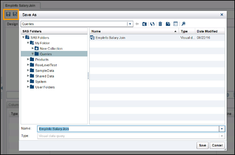
After you save the query, it shows up in the metadata folder structure on the left side where you put it. When you save the query, we can see the metadata object in the LASR Analytic Server. You can view what is in the LASR Analytic Server by clicking the home menu in the top left corner and selecting Administrator. The Emp_Salary table has a red square for its status because there is not yet data associated with it, just its definition.

7.   Click ▶ in the menu bar of the Data Builder and then select Run.

The ▶ icon opens to a drop-down menu that gives you the option to preview or run the query. The Preview option runs the query and loads the first 100 rows into a temporary table so that you can review the output. The Run option loads the full data set into its output location. Both options show the data in the Results tab.

You can see the labels of the columns by clicking the Headings drop-down menu. Now, if you go back into the Administrator, you can see your data loaded with a green circle as its status.

Modify the query

Once you add all of the columns from the source tables that you want as output, you also have the ability to create new columns based on the data from the source tables. Notice that there are categories for character, numeric, and date in the type field. This is how each data item will be classified in the output table. If there is a data item that is not correct, you can change it.

You can also create custom calculations by using SAS functions on the input data tables that you have brought in or add new categorical data based on ranges or values in your data. SAS functions are a way to use the SAS language within the query to take action on data items. They can be used to parse out strings, manipulate dates, change case on characters, along with many others actions.

Adding a numeric calculation

One of the things that we want to look for is employees that have at least 25 years of experience. We have brought in BEGDATE, which is the date that they started, but we still need to calculate the time. A custom expression can help us out.

To add a numeric calculation using functions:

1.   In the Column Editor, click the plus sign icon on the last row to add a new row. Give the data item a name, type, and label.

2.   In the Expression field, click the icon at the end of the field.

3.   Calculate the employee’s length of time with the company using TODAY() – BEGDATE.

The expression window has a tabbed panel on the left and the SQL expression on the right. You can choose to type the SQL statement or double-click from the Fields and Functions on the left. The columns from the input tables are under fields. You can find the Today function under Date/Time Manipulation in Functions.

Note: With SAS date functions such as Today(), SAS handles them by converting dates to integers based on 0 = January 1^st, 1960. Any dates before then are treated as negative integers.

4.   Click Apply to return to the Column Details window. Here you can click Verify in the top toolbar next to the Save and Save As icons. The verify feature checks your code for any syntax errors.

5.   Click Preview to see the results.

The result is shown in days. It would be easier to understand if it was in Years. Let’s modify the formula so that the result shows in years.

6.   Edit the expression in the Expression field. In the expression field, divide by 365. Then change the format to 8.

Note: A format of 8. shows the numeric field with up to 8 digits and no decimals. Adding a digit after the period allows for any decimal digits up to that digit.

7.   Run the Preview to see the results.

Adding a character data item

We want to plot the states to view our dedicated employees’ general locations. Our ADD2 data item has the city, state, and ZIP code of their addresses, but we’re only concerned about the state. Using the expression window, we can also use functions on character data to create new columns.

To add a new character column using functions:

1.   Add a data item and open the Expression Window.

2.   On the Functions tab, go to String Manipulation and double-click the SCAN function.

3.   On the Fields tab, select EMPINFO.ADDR2. This is your string.

Note: The SCAN function in SAS delimits a string into sections based on a certain character and extracts the section that you want. In the SQL expression, the SCAN function is shown as SCAN(string, section to extract, ‘delimiter’).

Since our address field is shown as “City, State, Zip” we are going to have to use a SCAN within a SCAN to extract our two letter state.

4.   Preview your data again. You can see that now you have the State data field.

Here are some other useful SAS functions for your data prep. *For all available SAS functions, please visit support.sas.com.
STRIP(var)	Removes leading and trailing blanks.
TRANWRD(var, target, replacement)	Replaces specific text (target) with text of your choice (replacement).
COMPRESS(var, text)	Removes elements (text) from your character string.
SUBSTR(var, start position, length)	Extracts a substring from your character string. You can identify the spot (start position) and how many characters to extract (length).
CAT(var1, var2, … varN)	Combines strings. Other variations let you identify a delimiter or how to handle blank spaces. CATS trims all leading and trailing blanks.
UPCASE(var)	Converts all characters in the string to uppercase. LOWCASE and PROPCASE are also functions that can be used to change case.
PUT(var, format)	Changes variable type from numeric to character.
INPUT(var, informat)	Changes variable type from character to numeric.

Filtering the data

There are two ways to filter the data in a data query. Behind the scenes, this is a SQL query, so the WHERE and HAVING clauses are used to filter out what you do not want. A WHERE clause specifies conditions on the input data to filter out before anything is even processed or calculated. The HAVING clause filters out values after processing, which allows it to handle both input data and any aggregate functions or new columns.

Adding a WHERE clause

We only want active employees. The easy way to get this information is to just get those who did not have an end date. From there, we can use a WHERE clause to filter out those with an end date.

To add a where filter:

1.   Go to the Where tab. This tab enables you to add the WHERE clause.

2.   On the Fields tab, drag the ENDDATE data item to the SQL expression box.

3.   Click the ENDDATE values at the bottom of the Fields tab to see a list of values to filter. Click the missing (.) check box.

4.   Preview the result.

Adding a HAVING clause

Going back to our original reason for querying this data, we only want to see employees with around 25 or more years of experience. We can use the HAVING clause to filter those rows out after we have already made the calculation for the dates since the HAVING clause works as you are exiting the data source.

To add a HAVING clause:

1.   Go to the Having tab.

2.   Find the Emp_Length data item. On the Fields tab, this time you have an Output Columns section. Expand it to see the columns set for output. Drag Emp_Length to the SQL expression panel. Notice how it used the formula instead of the column name.

3.   Add the >= 25 at the end of the formula.

4.   Run Preview. Now you see only rows with Emp_Length at or longer than 25.

Create a summary data query

In the previous example, we explored how the Data Builder gives you the ability to combine, filter, and calculate on incoming data sources. Using the power of SQL, the Data Builder can easily summarize data for you. This means taking a certain measure and calculating a statistic on all of the rows of the data set. The Data Builder has a standard set of aggregate functions that you can use on the Inputs tab.

When using these aggregate functions, you can also base these statistics on a certain data item in the data set and only aggregate on the distinct values of that data item. This is referred to as using a Group By.

Here are the basic summary statistics available in the Data Builder:

•   Count

•   Average

•   Sum

•   Minimum

•   Maximum

•   Standard Deviation

Steps to summarize data

For this example, we are going to use the same tables in the previous query. We want to look at salaries based on the company’s locations as well as the gender of employees working at each location. For this, you start a new query, drag the EMPINFO and SALARY tables into the Design tab, and then add LOCATION, GENDER, and SALARY to the column editor.

To add aggregations to the data query:

1.   On the Inputs Tab, select SALARY as the table from the top drop-down list.

2.   In the Default Aggregations section, under the Auto-Aggregate field, select Enable.

3.   Click the … button in the Default Aggregations field and select the Pick aggregations.

4.   Go to the Output Columns tab in the bottom section. Notice how the Salary field has now been broken into all of the aggregations that we specified in the previous step. Now preview the data.

You can see here that for each of the aggregations for Salary, we are getting the same number in each row. This is how an aggregation is done without a Group By. All of the rows are calculated on, and a new column is added for the calculation with the same value being issued for each row. This can be useful in some instances, but it is not what we’re looking for in this data set.

5.   Go back to the Column Editor on the Design tab. Under Aggregations, click the button for Location or Gender, select Group By, and then Apply.

6.   Run the preview.

This time we only get 9 rows of data. That’s because we grouped by Location and Gender. Therefore, we get only one row for each of the combinations of Location and Gender available in the data. Then for each one of those combinations, the aggregations are computed. Each of the numbers for the aggregations are based on just the rows that match that Location and Gender.

Updating the code

When you are working in the Data Builder, the application is building SAS and SQL code behind the scenes to develop each query. You can see the results of each of your options by going to the Code tab that’s right next to the Design tab. An example is shown below in the following figure.

Figure 4.3 Data Builder layout

Each time you make an addition, change, or selection in the Data Builder, the tab contents are updated with the corresponding code. If you scroll through it, you see LIBNAME statements, PROC SQL statements, macros for registering tables, and so on. This is all written in the SAS language, so it is possible to copy this code and run it in SAS Enterprise Guide or use it in a batch process.

The Preprocess and Postprocess links are to blank editors of code where you can put additional SAS statements that run before or after the query runs. For example, if you had another library that you wanted the query to write to, you could have a SAS statement that sends it there as well. You can use the Validate icon at the top to check your SAS statements as well.

Scheduling a query

The Data Builder also lets you automate queries through a scheduling feature. This is useful when you have reports that need the data refreshed hourly, daily, monthly, and so on. Within the scheduler, you can also choose if you would like to run it just once or make it a recurring event.

The scheduling feature works by creating a job, deployed job, and deployed flow that get stored in the same location as the query. The job takes care of the data query processes. A deployed job is then created from the job, which places that job into a deployed flow. This is all then scheduled on the scheduling server from the Data Builder. (See the SAS Visual Analytics: User’s Guide.)

Figure 4.4 Schedule window

In Figure 4.4, you can schedule a job by clicking the clock icon in the top toolbar of the query. Once the icon is clicked, a schedule window appears.

In this window, you can either Run now, which immediately executes the query, or you can Select one or more triggers for this query, which is where you can create a Time Event.

A Time Event enables you to schedule the query at a future time and also decide whether you want this to recur on an interval. For this example, we are going to create a Time Event that runs the query at 6:00 AM every weekday.

Figure 4.5 New Time Event window

After running this more than once and on a daily schedule, the options appear in the central window to decide on the time. Interval in days lets you choose to run it on different days. So if you wanted to run it every other day, you would select that choice and increase the number to 2. We want this to run every weekday, so that is what is selected. In the next window, you can choose the time. Duration in minutes at the bottom is where you can declare how long to wait on dependencies if they are involved in your process. So if this query is waiting for another job to complete or file to be created before processing, you can set the number of minutes that it waits for that condition to be met. Then at the end, you can choose when this scheduled query starts and ends.

References

SAS Institute Inc. 2016. SAS Visual Analytics 7.3: Administration Guide. Cary, NC: SAS Institute Inc.

SAS Institute Inc. 2015. SAS Visual Analytics 7.3: User’s Guide. Cary, NC: SAS Institute Inc.