As already emphasized, in Spotfire, the data loaded into data tables is crucial for successful visualization creation. It must be in a workable format (or a format suitable for aggregation) as Spotfire's data table data manipulation capabilities are somewhat limited.
This does not mean, however, that Spotfire cannot perform some work on the loaded data. The tool has the following loading and transformation capabilities:
- Data loading: It includes:
- Adding a data table
- Inserting data table columns
- Inserting data table rows
- Data transformation: It includes:
- Pivoting the data
- Unpivoting the data
- Calculating and replacing the column
- Calculating a new column
- Changing the column name
- Changing the column data type
- Replacing data table
All these capabilities will be described in the following sections.
This topic was already presented in the Data loading section of Chapter 3, Creating Visualizations. The theory was accompanied by the demonstration of loading from one of the three different data source types: text file, MS Excel file, and database.
Spotfire Professional allows its user to load extra (or new) columns to an already existing data table.
This is useful due to the fact that the visualizations have only one main data table. The records of main data tables are the base for the creation of graphs, defining rows in nonaggregated visualizations, and items in aggregated ones.
Users are able to insert new columns from a second data source, extending the original data table. More importantly, the second data source can be totally unrelated to the first data source (of the already loaded data).
To add a new column, please access the menu Insert | Columns. If more than one data table exists in the analysis, a dialog box will be launched for the user to choose the table to which add the columns (dialog box Select Destination). In our case, we will select Employees. After clicking on Next, the dialog box will allow the user to configure the data source, as shown in the following screenshot:

We will add the columns from the JOBS table of the hr database schema; the configuration steps are identical to the Loading from Databases scenario previously described in Chapter 3, Creating Visualizations.
After configuring the source, the user will be presented with the Match Columns dialog box (here we should configure the matching columns between both tables). The Match All Possible option handles this task for us, as in our case, both columns to relate share the name and can be automatically identified by the application.
Refer to the following screenshot where the Column Match dialog box is depicted:

By clicking on Next, the user is moved to a column selection dialog box; although several columns were selected while loading the data source, the user might not wish to add all to the existing data table. In our case, we will select JOB_TITLE (refer to following screenshot for details).

There are also some options related to the definition of which data is going to be included in the resulting data table—Join method. We will leave the default option.
Clicking on Finish terminates the dialog box and imports the data.
Tip
To confirm the new column, we can go to the menu View | Data. A new panel is opened on the left-hand side of the screen. Choosing the data table Employees will reveal that there is in fact a new column.
To further analyze the data, it is also a good idea to create a new page with a new table visualization. Besides the job ID, there is now also a job description column.
Adding rows to a data table is very similar to adding columns to a data table. And also, as happens for columns, this feature serves as a solution for extending any main data table that exists in the analysis.
The added rows need to match the existing data table columns if automatic matching is to be done. If not, manual matching has to be performed.
Create the following MS Excel worksheet so that we can import the data:

To add new rows, access the menu Insert | Rows, and we will use the data table Performance as the destination for the new rows.
The automatic matching of columns (from the Match All Possible button) will only work for Race. All other columns have to be matched by hand as the names differ. The resulting matching should be similar to the following screenshot:
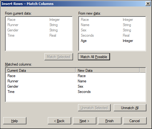
Since Age (or similar) does not exist in the Performance data source, we will not include this column. Its addition would lead to the creation of empty column values for the records already in the Performance data table.
While loading data into Spotfire, the user is allowed to modify it. The aim of this feature is to permit users to clean up the data, fix data errors or omissions, or even change formats and types of the columns.
This task has to be specified while loading the data, which as specified previously, occurs solely in the following scenarios: Add Data Tables, Insert Data Table Columns, Insert Data Table Rows, and Replace Data Table. Then, the transformations have to be defined in the Add Data Tables dialog box. Refer to the Transformations section on the following screenshot:

A pivot table in Spotfire has the same meaning as in MS Excel. The purpose of these tables is to summarize the data.
This transformation mutates a tall and skinny data table into a short and wide one, where the new columns are usually comprise of aggregated values.
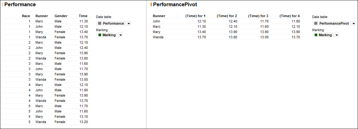
As an example, we will pivot the data of Performance into a new PerformancePivot data table.
It is during the creation of the data table, that the user will have the opportunity to define its pivot transformation. Our aim will be to pivot [for each Runner] Time per Race (without any selected aggregation function).
To achieve this, follow these steps:
- Start by creating a new data table named PerformacePivot, by loading the Performance Excel worksheet. From the Transformations drop-down list, select the Pivot option and click on Add. A dialog for the Pivot definition will be presented as shown in the following screenshot.
- Define Runner as Row identifiers (for each runner), Race as Column titles (per race), and Time as Values (value of the records).

Comparing the pivot data table with the original format, we can easily visualize the transformation from tall and skinny to short and wide (both tables are shown side-by-side in the following screenshot):
Unpivoting a table transforms it in the opposite way of pivoting: from short and wide to tall and skinny.
As an example, we will unpivot the StoreSales data into a new StoreSalesUnpivot data table.
The procedure to unpivot data is similar to the procedure to pivot data; a new data table needs to be created with an unpivot transformation. Our objective will be to unpivot the sales department (Furniture, Toys, and so on) into a Department Id column, and department totals in a Department Total column.
To achieve this, please create a data table named StoreSalesUnpivot loading the StoreSales.txt file. Choose transformation of the type Unpivot and define the transformation as presented in the following screenshot. The meaning of the unpivot configuration is as follows:
- Columns to pass through: It lists the columns that are not affected by the transformation, but which will exist in the new data table.
- Columns to transform: It lists the columns that are to be merged in a single category column. In our example, we will unpivot the several departments (Furniture, Toys, and so on) into a single column named Department Id.
- Available Columns: It defines columns that will not exist in the new data table.
- Category column name: It defines the name of the new category column.
- Value column name: It defines the aggregated value for the result of transforming multiple [
integer] rows into one category row. This value is calculated by aggregating the different values from the excluded columns. In our example, this value is the result of adding the department total for the several distinct records of: Customer age, Date joined, First buy, Recency, Number of purchases, and Receipt average.
Note the Department Id and Department Total columns are the new unpivoted columns.
Spotfire allows users to replace columns with others whose values are calculated through the use of an Expression. This transformation is known as Calculate and Replace Column, and as it happens with all the data transformations, it can only occur on data loading.
The Calculate and Replace Column dialog box offers users several customizations, such as Column to replace, Available columns (to use in the expressions), Functions (to create the expressions), Expression builder, and also various Formatting options.
The following screenshot demonstrates the creation of a column named Date joined span, which replaces Date joined (for the StoreSales data). This new column contains the difference between now and Date joined in days.

The calculated column will have values as shown in the following screenshot:

The difference between the transformations Calculate New Column and Calculate and Replace Column is solely that the first adds a new column to the data table, while the second replaces a column in the data table.
In terms of configuration, both behave in the same way, each having the same rich feature set.
Change Column Names is one more transformation available for the user. The new column name does not need to be a defined hardcoded value, as it can also be calculated using the Expression builder.
The following screenshot displays the available functions for building a new column name.

The default data type of a loaded column can also be manipulated: Date columns can be loaded as Strings, Integer columns can be loaded as Currency, and so on.
The formatting of the columns is also possible, as the application provides a very rich set of formats. The following screenshot lists the available formatting options of a Date category.
Besides some predefined possibilities, the user can inclusively define a format from scratch using the Custom format.

In some scenarios, the users might want to keep one or more visualizations, but replace the underlying data with a new set. An example of such a case could be a consulting company that analyzes their quarterly results through a set of custom visualizations. It is expected that at the end of every quarter, they will want to load the quarterly data into Spotfire and run the analysis on the new data.
For such cases, Spotfire Professional offers the possibility of replacing the data table content. Users just need to provide a new set of data which has the same columns with the same data types as the original data.
To experiment with this function, navigate to the menu File | Replace Data Table. A dialog box named Replace Data Table – Select Data Table will be displayed, as shown in the following screenshot:

In the Select data table to replace: dropdown, users are able to select the data table in which they want to load the new data, while the Replace with: radio button provides extra loading configuration options.
So far we have seen the creation of visualizations from a single data table. This is the most common task; however, the tool is not limited to it. If this limitation existed, it might lead the users to create massive merged tables, full of repeating data, instead of the traditional relational data models.
The Spotfire feature Column Matches, enables the matching of columns between distinct data tables, thus fostering the use of multiple data tables in a single visualization. In this aspect, Spotfire is extremely friendly, as it makes two matching modes available: automatic and manual.
Spotfire considers that the two columns match when the names and data types match. This is not always necessarily true, however; matched columns are not necessarily connected and hence do not need to be leveraged.
To access the analysis's Column Matches, navigate to menu Edit | Data Table Properties and a dialog box will be shown. Accessing the tab Column Matches displays the matched columns for each of the selectable data tables.
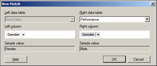
The following screenshot lists the automatic matches for the StoreSales data table:

This match is actually incorrect as the data tables are unrelated, and therefore we should delete it. To delete it, select the match in the current matches list and click on the Delete button next to the list. Now, our data tables are no longer connected.
If Spotfire does not identify the columns as matching, the user can force this, by defining new matches.
To do so, users should click on the New button in the Data Table Properties dialog box (the Column Matches tab), and select both the data table and the columns to match as shown in the following screenshot:
Relations are the ties between columns of two distinct data tables. They are similar in principle to Column Matches but their function is different; their aim is to propagate filtering and marking between visualizations.
For instance, if two visualizations have defined a relation between two columns of their data tables, marking data in the first visualization will mark related records in the second visualization.
The columns chosen to participate in a relation should be identifier columns in both the data tables, and more than one column can be related between two data tables.
To exemplify the creation of a relation between two data tables, we will first need to import new data. Add the table JOB_HISTORY (from the Oracle XE database and user hr) as an analysis data table named JobHistory. Before closing the Add Data Tables dialog box, make sure you click on the Manage Relations button to add a relation to data table Employees. Refer to the following screenshot for the Manage Relations dialog box:

Click on New and the New Relation dialog box will be opened. Refer to the next screenshot for details:

To configure a new relation, perform the following steps:
- Define the Employees data table as Left data table: and leave EMPLOYEE_ID as Left column:
- Define the JobHistory data table as Right data table: and leave EMPLOYEE_ID as Right column:
- Click on OK.
A new relation is now created between Employees.EMPLOYEE_ID and JobHistory.EMPLOYEE_ID, which is displayed in the Manage Relations dialog box shown in the following screenshot:

Click on OK twice to close the remaining the dialog boxes. You may also close the default scatter plot created for the new JobHistory data table.
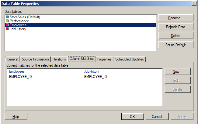
Going back to the Data Table Properties dialog box, and validating Column Matches of the data table Employees, you can verify that three new Column Matches were created between the data tables Employees and JobHistory: DEPARTMENT_ID, EMPLOYEE_ID, and JOB_ID. Remove DEPARTMENT_ID and JOB_ID, as only EMPLOYEE_ID is a linking key between the data tables.
By deleting the match on the Employees data table, the symmetrical match (from JobHistory to Employees) will also be removed.
The following screenshot displays the Data Table Properties dialog box with the final result: