You have already seen that the most relevant function used when applying aesthetic mapping is the aes() function. Leaving aside the mapping of the x and y variables, which were already covered in the previous chapter, we will now focus on the other mapping options. The most useful attributes to map are the color, the type of line, or the symbol used to represent the data (linetype or shape respectively, size of the symbols, and transparency (alpha). All these attributes can be mapped to different variables and combined in the plot in order to get the required data representation or the visual effect. In the examples we have come across until now, you have already seen some applications of the mapping for colors. The same approach can also be applied to the other attributes.

In the following example, we will create a dataset with three series of exponential values using exponents of 1, 1.5, and 2, and we will plot these three series of data. In the dataset, we will also include, together with our x and y values, a flag, which will allow us to retrieve the three different sequences of data, and we will use this flag to map the data. The following code shows this:

cont <- data.frame(y=c(1:20,(1:20)^1.5,(1:20)^2), x=1:20,group=rep(c(1,2,3),ea
ch=20))

We will represent the different sequences of data as points or lines using the geom_point() and geom_line() functions. The following code shows this:.

#### Data represented as points
ggplot(data=cont, aes(x=x, y=y, col=factor(group)))) + geom_point()
ggplot(data=cont, aes(x=x, y=y, col=factor(group),size=factor(group))) + geom_point()
ggplot(data=cont, aes(x=x, y=y, col=factor(group),shape=factor(group))) + geom_point()

#### Data represented as lines
ggplot(data=cont, aes(x=x, y=y, col=factor(group))) + geom_line()
ggplot(data=cont, aes(x=x, y=y, col=factor(group),size=factor(group))) + geom_line()
ggplot(data=cont, aes(x=x, y=y, col=factor(group),linetype=factor(group))) + geom_line()

As illustrated, we first assigned the grouping factor to the color attribute, we mapped the size of the line or points, and then we mapped the type of symbol used. In this last case, you would notice how we have used different arguments since point symbols can be mapped using the shape argument, while the tile of the line can be mapped with the linetype argument.

In Figure 4.9, you can see the plots we have obtained:

Figure 4.9: These are examples of points (left) and lines (right) with aesthetic mapping of colors (first row), size (second row), and type (third row)

You would also notice how, with the mapping size (second row of Figure 4.9), the aesthetic maps, by default, the size to the value of the mapping variable (group in our example). Consequently, group 3 has much bigger points and thicker lines compared to group 1.

In the next section, we will have a look at the mapping of the alpha parameter, which adds transparency to the element of the plot.

In the previous chapter, we described how the stat_x functions work in general: they take the data you provide as input, and they use such data for statistical calculations. During such calculations, new variables can be created, such as the variable defining the bins or the variable defining the count element in a histogram. The output of these statistical transformations is also a dataset that contains the original data and the new variables created in the process, and that depends on the specific stat_x function used. In Chapter 3, The Layers and Grammar of Graphics, you can find a summary table for these stat functions that also contains specific new variables created for the most important functions. These newly created variables are quite interesting since they can also be used in the plot that contains the stat_x function. This is exactly how the results of the statistical transformations are represented in the plot. On top of this default representation, you can also use these newly created variables to represent additional information on the plot, or you can, for instance, map aesthetic attributes to such variables.

We will now just see a simple example showing how we can use such variables which, in some cases, can produce a very nice effect on the histogram, for instance. We will just create a simple normal distribution with default values (0 as the mean and 1 as the standard deviation) using the rnorm function, and then we will create a histogram of such a distribution. We can then map the filling color to the number of observations in each bin available in the new count variable created by the stat_bin() function. Just remember that, in order to avoid errors because of variables with the same name in the original dataset, the newly created variables must be surrounded by .., so in our example, we would need to use ..count... The following code shows this:

set.seed(1234)
x <-data.frame(x=rnorm(1000))
ggplot(data=x, aes(x=x, fill=..count..)) + geom_histogram()

Since we are performing a simulation of random numbers, as the first thing, we set up the seed function used in the random number generation process so that we get the same results every time we run the code. The plot we just obtained is represented in Figure 4.10. As illustrated, the use of such variables is quite similar to the traditional variable; the trickiest part is to know which additional variables you have available for the statistic you are using, and for this, you can use the tables in the previous chapter. With them, you can also get new ideas about new applications that better fit your needs.

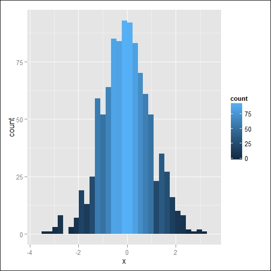
Figure 4.10: Here's a histogram of a normally distributed random variable representing the data count (default option) with the color intensity proportional to the data count

Applying this method to aesthetic mapping, we use a continuous scale of color tones to map the observation count. Since the scale is continuous, we cannot apply this method on geometries with only one continuous plot area, such as geom_density(), which generate a smooth estimate of the kernel density. We have used this function in some of the examples in Chapter 2, Getting Started.

On the other side, you can apply it to the histogram representing the density of observations. We can, in fact, use the new variable density created by the stat_bin() function to represent as a y value the density of observations present in each bin and at the same time use a filling color proportional to the observations. The following code shows this:

ggplot(data=x, aes(x=x)) + geom_histogram(aes(y=..density..,fill=..density..))

We can also combine multiple geometries on the same plot and also add the kernel density function on top of the histogram we have obtained. The following code shows this:

ggplot(data=x, aes(x=x)) + geom_histogram(aes(y=..density..,fill=..density..)) + geom_density()

You can see both plots in Figure 4.11. You can see how the data density is scaled to integrate to 1 and how in this case we have used the new variable ..density.. not only for the color filling aesthetic, but also for the plotting value y. In the previous example, when representing the data count, we did not need to specify the y variable since the default behavior of geom_histogram() is to represent the data count.

Figure 4.11: (A) This is a histogram of a normally distributed random variable representing data density with color intensity proportional to the data density scaled to 1. (B) This is the same plot as (A) but also includes the estimate for the kernel density function

As you can see from the plot in Figure 4.11, the graphical effect that we have produced with this mapping is to have the data bins represented with a color shade that is proportional to the amount of data in each bin. A similar effect can be obtained by assigning a mapping to the alpha variable, which defines the transparency of the data. We have already used the alpha attributes in some other examples previously, but in this case, we will use it for an actual aesthetic mapping instead of assigning a fixed value to it. This means that we will need to give the definition of alpha in the aes() function, together with the other aesthetic attributes. The following code shows this:

ggplot(data=x, aes(x=x)) + geom_histogram(aes(alpha=..count..))

As illustrated in the resulting plot in Figure 4.12 (A), the default behavior of alpha mapping is to use gray scales since it is not a mapping of colors but rather a mapping of transparency. It is also possible to combine the mapping of the previous example with the filling, together with the transparency, and you can see the resulting plot in Figure 4.12 (B). The following code shows this:

ggplot(data=x, aes(x=x)) + geom_histogram(aes(alpha=..count..,fill=..count..))

As is apparent, the effect is quite redundant since both mappings produce a similar effect although one is based on color and the other on transparency. You would also notice how the two mappings are considered independent and ggplot2 will produce two different scales for them.

Figure 4.12: (A) This is a histogram of a normally distributed random variable representing the data count with transparency (alpha) mapped to the data count. (B) This is the same plot as (A) but also includes a filling mapping to the data count

If you want to try out such a mapping on real data, you can go to Chapter 2, Getting Started, where we used the iris dataset as an example for histograms and density plots. You could, for instance, add alpha mapping to Figure 2.4 of Chapter 2, Getting Started, with the following code:

ggplot(data=iris, aes(x=Petal.Length,col=Species,fill=Species,alpha=..count..)) + geom_histogram()

In the preceding chapter, in Figure 3.4, we saw an overview of a few options of scales and the difference in scales between continuous and categorical variables. In this section, we will have a closer look at how the assignment of scales is done using these different scales and at how you can control this aspect to get a grip on the scale that is used.

Let's first create a small dataset with four different distributions of random variables:

dist <- data.frame(value=rnorm(10000, 1:4), group=1:4)

The distributions we just created are all normal with a standard deviation of 1 but are built around an increasing mean, so the first distribution will have 1 as the mean, the second will have 2 as the mean, and so on.

We can plot such data as jittered points using a different color for each group; with the following code, we obtain the plot in Figure 4.13:

ggplot(dist, aes(x=group, y=value, color=group)) + geom_jitter(alpha=0.5)

As illustrated, we simply represented the values of the distributions on the y axis for the different groups that are on the x axis. As shown, the default scale selected by ggplot2 is a continuous scale where the color intensity is associated with the color value. Of course, this is not what we are interested in since we just wanted to represent the different distributions with a different color that is easy to identify and not connected in a color scale. The reason for this is related to the type of values that we represented.

In fact, in our dataset, the variables contained in the group column are numeric, and this means that ggplot2 will treat them as connected in a numeric scale and consequently will associate with them a continuous scale. One way to overcome this issue is to simply change the variable to factor. In this way, the numbers will be treated only as levels and not as numeric values.

Figure 4.13: This is a representation of different distributions with jittered points

This can be done, of course, directly in the dataset in simple examples as ours, but in most cases, where, eventually, you will use a big dataset, you would not want to change its variables for each plot. In this situation, it is much more convenient to change the variables directly in the plot. The following is the code to have the grouping variable as a factor:

ggplot(dist, aes(x=group, y=value,
color=as.factor(group))) + geom_jitter(alpha=0.5)

In Figure 4.14, you can see the resulting plot. As illustrated, changing the variable to factor will produce a default plot with the as.factor(group) scale notation. This can be changed by changing the title of the legend; we will see how to do that in the next chapter. The use of converting a variable from numeric to factor can turn out to be very handy, and I am sure that you will find this approach when browsing for help. In the following code, you can find an example of such an approach on a real dataset—the mtcars dataset. In this case, the grouping variable, that is, the number of cylinders of the cars, is also treated as numeric, but the idea is, of course, to simply use this variable as a grouping variable. The following code shows this:

ggplot(mtcars, aes(mpg, wt)) + geom_point(aes(color = cyl))
ggplot(mtcars, aes(mpg, wt)) + geom_point(aes(color = factor(cyl)))

Figure 4.14: This is a representation of the different distributions with jittered points and with the grouping variable treated as a factor

In this section, we will take a look at some of the most useful annotations you would want to add to a plot. After you have represented your data, you would probably need to add a specific reference to the plot, for instance, vertical bars, text, or other types of annotations. The ggplot2 package provides a vast variety of options, and for a complete reference, you can have a look at the ggplot2 documentation website http://docs.ggplot2.org. In this section, we will take a look at the most important annotations.

Let's consider again our dataset that we created previously just by generating a series of normally distributed random numbers.

x <- data.frame(x=rnorm(1000))

We can, for instance, represent this distribution using a histogram. In this case, it could be useful to add a vertical bar to the plot representing the mean of the distribution. As for graphics, ggplot2 also provides three major functions to produce such reference lines:

The first two functions are a special case of this last one since they allow you only to represent lines parallel to the axis. In the following code, we use the relative function to add a vertical line to the histogram corresponding to the median of the distribution:

ggplot(x, aes(x=x)) + geom_histogram(alpha=0.5) + geom_vline(aes(xintercept=median(x)),
color="red", linetype="dashed", size=1)

We also specified the color, the type of line, and the size the line should have. You can see how such arguments are similar to the arguments used by other graphical packages in R. As you have seen in this case, we specified the intercept on the x axis by calculating it from our data. This is a very useful approach since even if you changed the data, the plot would still be produced correctly. Of course, as an alternative, we could also specify the numeric value at which we want to have our intercept. For instance, we can add to our plot a horizontal line corresponding to a level of 50 in our data count. In this case, we will draw a solid black line:

ggplot(x, aes(x=x)) + geom_histogram(alpha=0.5) + geom_vline(aes(xintercept=median(x)), color="red", linetype="dashed", 
size=1) + geom_hline(aes(yintercept=50), col="black", linetype="solid")

You can see the resulting plot in Figure 4.15:

Figure 4.15: This is a histogram of a normal distribution with two reference lines

Together with the vertical line, it is also possible to add text to the plot as an annotation. Text as well as lines can also be mapped to variables, producing a plot representing text corresponding to the variables, for instance. In this case, it would be nice to include in the plot an indication that the red vertical bar refers to the median and specify its numeric value. We can do that using the geom_text() function, in which we can specify the text we want to add as well as its coordinates. The following code shows this:

ggplot(x, aes(x=x)) + 
geom_histogram(alpha=0.5) + geom_vline(aes(xintercept=median(x)), color="red", linetype="dashed", 
size=1) + geom_hline(aes(yintercept=50), col="black", linetype="solid") + geom_text(aes(x=median(x),y=80),label="Median",hjust=1) + geom_text(aes(x=median(x),y=80,label=round(median(x),
digit=3)),hjust=-0.5)

Within the geom_text() function, we also used aesthetic mapping to define the position of the objects. As you can see, we had the possibility of using a numeric value as we did for the y argument, as well as a calculated value as we did for the x value, which is calculated using the median() function. In this situation, when you actually don't know the value but you calculate it within the plot function, it is very useful to use adjustment arguments to add an offset to the text so that it does not overlap with the median line. You can do that using hjust for horizontal adjustment and vjust for the vertical ones. These adjustments will represent the text with a shift from its original position equivalent to the value that you provided. In our example, the word "Median" will be shifted by 1 unit to the left, while the numeric value of the median will be shifted by 0.5 to the right since the value is negative. Since the default of the digits produces a number with too high a level of precision, you would often need to round off these calculated values, and that's what we did using the round() function, in which we specified the number of digits to represent.

Finally, ggplot2 also provides an annotate() function that allows you to easily create annotations to the plot. You can use it to add specific lines, text, and a shading area to the plot by providing the limits on the axes. You would find an idea of the possible annotation by looking at the help page of the function or on the ggplot2 website. Additional examples are also shown on the ggplot2 website under the theme() function. In this case, we will have a look at one example. We will draw a shade area on our histogram covering the interquartile range between the twenty-fifth and the seventy-fifth percentiles.

The following code shows this:

ggplot(x, aes(x=x)) + geom_histogram(alpha=0.5) + geom_vline(aes(xintercept=median(x)), color="red",linetype="dashed", size=1) + geom_hline(aes(yintercept=50), col="black",linetype="solid") + geom_text(aes(x=median(x),y=80),label="Median",hjust=1) + geom_text(aes(x=median(x),y=80,label=round(median(x)
, digit=3)),hjust=-0.5) + annotate("rect", xmin = quantile(x$x, probs = 0.25), xmax = quantile(x$x, probs = 0.75), ymin = 0, ymax = 100, 
alpha = .2, fill="blue")

As illustrated, in the annotate() function, we selected the type of geometry we want to represent, that is, the rectangular one, and then we defined the extremes of the area. You would also notice that since, in this case, we are not mapping aesthetics, for our calculations, we need to provide a specific reference to the dataset, for instance, in quantile(x$x, probs = 0.75), we need to specify the actual column in the datasets. On the other hand, for the calculation of the median, within the aes() function, we were able to specify only the column in the dataset since the data was already loaded in the plot object ready for aesthetic mapping. You can see the final plot with all our annotations in Figure 4.16:

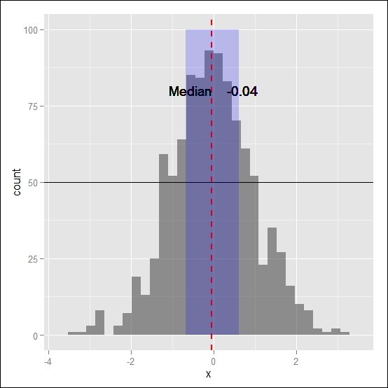
Figure 4.16: This is a histogram of a normal distribution with two reference lines, the notation for the median value, and a shade area for the interquartile range

The annotate() function can be very useful to quickly make annotations without having the data in a data frame structure, for instance, in this case, we were able to draw a rectangular area without the need to have to use geom functions.

Add text and reference lines with facets

In the examples we just discussed, we applied text and reference lines to only one plot, but in many cases, you would probably have plots divided into facets in which you would also like to add reference lines. One easy way to do that is using the same approach we discussed in the Adding statistics section at the beginning of this chapter. We can add text as well as the reference lines by applying the layer to only a subset of data. We can see an example of this using the dist dataset, which we created in the previous sections, and which contains four different normal distributions. We will represent such distributions in facets, and we will apply a reference line on the median value of the first distribution as well as its numeric value. The following code shows this:

ggplot(dist, aes(x=value, fill=as.factor(group))) + geom_histogram(alpha=0.5) + geom_vline(data = subset(dist, group 
=="1"), aes(xintercept=median(value)), color="black", 
linetype="dashed", size=1) + geom_text(data = subset(dist, group 
=="1"),aes(x=median(value),y=350,label=round(median(value), digit=3)),hjust=-0.2) + facet_grid(.~group)

As you can see from the preceding code, we simply applied the text and the vertical line only to the data with the group value equal to 1. This way, we add these elements only to the first facet. You can see the resulting graph in Figure 4.17. You would also notice how selecting the data within the geom_text() and geom_vline() functions, the median is only calculated on this subset of data.

Figure 4.17: This is a histogram of the dist dataset with a facet for each distribution. A reference line indicating the median is added on the first facet and the median value is also included

Using the same approach, you can add the median reference line and the median value to the other facets; you will just need to also include the code for the other groups as well. On the other hand, you will get reference lines on the plots that will not match the colors used in the distributions since we include a component after the other instead of letting ggplot2 split the data and make the color assignments. To solve this, recall the default assignments of colors and then use them in the plot. We already mentioned in Chapter 3, The Layers and Grammar of Graphics, how equally spaced colors on the color wheel are assigned the default to categorical variables. Here, we will show a practical example of that.

First of all, we create a vector with the first four default colors assigned by ggplot2 to categorical variables. The following code shows this:

myColours <- scales::hue_pal()(4)

The myColours vector will contain the four colors in the same order as assigned by ggplot2, so the first will be assigned to the first variable, the second to the second one, and so on.

We will then create the plot using the same method used before with the difference that the colors used to draw the vertical line will be taken from this vector of colors. Since this code is quite long, you have the different parts of the code divided by a comment indicating to which facet it applies. You can also see italicized the code for the first facet since the remaining code will have a similar structure for the other facets. The following code shows this:

ggplot(dist, aes(x=value, fill=as.factor(group))) +
geom_histogram(alpha=0.5)+
### Facet 1
geom_vline(data = subset(dist, group ==1), aes(xintercept=median(value)), color=myColours[1], linetype="dashed", size=1.5)+geom_text(data = subset(dist, group==1),aes(x=median(value),y=350,label=round(median(value), digit=3)),hjust=-0.2)+
### Facet 2
geom_vline(data = subset(dist, group==2), aes(xintercept=median(value)), color=myColours[2], linetype="dashed", size=1.5)+
geom_text(data = subset(dist, group ==2),aes(x=median(value),y=350,label=round(median(value), digit=3)),hjust=-0.2)+
### Facet 3
geom_vline(data = subset(dist, group==3), aes(xintercept=median(value)), color=myColours[3], linetype="dashed", size=1.5)+geom_text(data = subset(dist, group ==3),aes(x=median(value),y=350,label=round(median(value), digit=3)),hjust=-0.2)+
### Facet 4
geom_vline(data = subset(dist, group==4), aes(xintercept=median(value)), color=myColours[4], linetype="dashed", size=1.5)+geom_text(data = subset(dist, group ==4),aes(x=median(value),y=350,label=round(median(value), digit=3)),hjust=-0.2)+facet_grid(.~group)

The resulting plot is represented in Figure 4.18. As you have seen, we now have the vertical reference lines with a matching color that is the same as the one used to fill the histograms, with a resulting nicer graphical effect. When using this approach, you just need to be sure that the reference lines can be clearly distinguished since you are drawing them on top of histograms having the same color. A possible solution, used in our example, is to slightly increase the size of the lines. In the final plot, you can also see how in each facet we obtain the same median calculation that was used to simulate the original distributions. Clearly, you could use the same method even to the text added to the facet by specifying the color in the geom_text() function.

Figure 4.18: This is a histogram of the dist dataset with a facet for each distribution. A reference line indicating the median is added in each facet with a color matching the ggplot default assignment