
As we mentioned in Chapter 3, The Layers and Grammar of Graphics, legends are guides that represent the inverse of the applied scales and are used to trace back the plot elements to the aesthetic mapping. For this reason, legends are defined in ggplot2 as guides since they represent guides to the aesthetic mapping. The legend that is created by ggplot2 depends on the aesthetic mapping and the geometry that is used in the plot. For instance, Figure 5.1 contains a continuous color scale, Figure 5.2 contains boxplots, and Figure 5.4 contains points.
Since legends are recreated by scale functions, most of the time you will need to use scale functions to modify the legend's appearance. In this section, we will go through how to change the four main aspects of legends: the title, labels, legend box, and legend position. But, first of all, let's see how we can remove the legend.
To remove the legend, you can use the guide argument of the scale function or directly use the guides() function dedicated to the manipulation of the guides. We will illustrate this using our boxplot example with the dist dataset:
### We create again our plot myBoxplot
myBoxplot <- ggplot(dist, aes(x=group, y=value, fill=group)) + geom_boxplot()

### Remove legend with guides function
myBoxplot + guides(fill=FALSE)

### Remove legend with scale function
myBoxplot + scale_fill_discrete(guide=FALSE)
As illustrated in the preceding example, the command is quite straightforward, and you can use the guides or the scale function to leave out of the legend by setting the aesthetic to false. For instance, in this example, we have used the fill aesthetic mapped to the group variable, so we will need to use the scale function for the fill mapping of the scale_fill_discrete() discrete variable, or the guides() function with the fill mapping set to FALSE. The result from both commands will be the same, namely a boxplot without a legend.
For all the legend adjustments we will go through in this section, it is possible to use both the guides() and scale functions, but we will only work with the scale functions in our examples since this has the greater functionality of the two and guides() is comparatively straightforward.
We have seen that the name argument of the scale function can be used for the axis label as well as the legend name. This may sound tricky but is actually quite simple. You will need to use the scale function for the aesthetic you want to manipulate. This aesthetic could be the axis, in which case the name argument will modify the axis label. Alternatively, the aesthetic could be the legend, in which case the name argument would modify the legend title. The following command shows a simple example of how to modify the axis name and the legend title, which will make this use clearer and generate the resulting plot of Figure 5.5:
myBoxplot + scale_x_discrete(name="This is my x-axis") + scale_fill_discrete(name="This is my legend")
This example modifies discrete variables in both cases; however, in the first case, we refer to the x aesthetic of the axis, while in the second case, the fill aesthetic is used to fill the boxplots with colors mapped to the group variable:
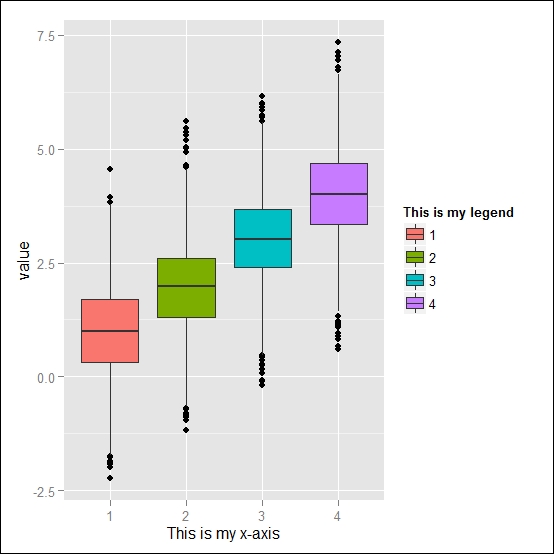
Figure 5.5: Example of boxplot with modified legend title and axis label
Not only can you use this method to change the legend title, you can actually remove it completely by simply providing an empty title name, as follows:
myBoxplot + scale_fill_discrete(name="")
As an alternative, you can also use the theme() function, as shown in the next command. However, in this case, you will remove all legend titles from all legends in your plot. We will look into the details of this function later on in this chapter. The following command shows this:
myBoxplot + theme(legend.title=element_blank())
The legend is composed of keys, the symbols relating the legend to the plot, and key labels, which describe what the keys represent. Generally, there are two main modifications to the default legend involving keys and key labels: first, to change the order of the elements, and next, to modify the text of the key labels. You can do these two modifications using the breaks and labels arguments of the scale function. The breaks argument defines which values appear in the legend, while the labels argument specifies the text that appears in the key labels. So, if you want to change the order of the keys in the legend, you can provide the order you want as a vector to the breaks argument. Just remember that the vector elements should match the dataset elements used to create the legend. The following command shows this:
myBoxplot + scale_fill_discrete(breaks=c("1","3","2","4"))
You can also directly inverse the order of the elements in the legend using the guide_legend() function. We have seen that the scale functions have an argument guide that can be used to control the legend's appearance and has the default value of guide="legend". If you would like to modify the legend's appearance, there are also other guide options that can be used, but you will need to pass the explicit function name to guide, so the default value would correspond to guide=guide_legend(), and in the function body, you can change the default assignments. This function allows you to have profound control over the legend's appearance. A full listing of all available arguments can be found on the help page of the ?guide_legend function. The guide_legend() function also provides the argument's reverse, which specifies that the legend order should be reversed. So, in our boxplot example, we could reverse the legend order with the following command:
myBoxplot + scale_fill_discrete(guide = guide_legend(reverse=TRUE))
The same approach can also be used with the guides() function, as shown here:
myBoxplot + guides(fill = guide_legend(reverse=TRUE))
In order to change the key labels, we can use the labels argument to provide a vector of names matching breaks. Here, you can see the resulting boxplot example with a modified order of the legend elements and updated labels:
myBoxplot + scale_fill_discrete(breaks=c("1","3","2","4"), labels=c("Dist 1","Dist 3","Dist 2","Dist 4"))
The resulting plot can be found in Figure 5.6:

Figure 5.6: Example of boxplot with a modified order of the legend key and legend labels