
8
Plate Torsion
In this section, calculations are made step by step, from the simplest to the most complicated, due to the complexity of the description of deformations.
8.1 Torsion of homogeneous cylinder
Consider a cylinder of length L along the torsion axis x. It has a radius R along y and z and a torsion test is applied, imposing a rotation by an angle θ; since there is no warping of the transverse section, the longitudinal displacement is zero. The two displacements v and w due to the rotation by an angle θ imposed by the torsion are v=-zθ and w=yθ. The following shears are generated:
In order to write the Lagrangian, an integration over the whole transverse surface of the infinitesimal volume element ds=2πrdr must be made with relation r2=y2+z2. Denoting by FT the torsion resonance frequency and by G the shear modulus, the deformation and displacement energies are:
The minimization of the Lagrangian yields:
The integration by parts yields the boundary condition and the vibration equation:
The vibration equation is therefore:
The boundary condition yields the eigenvalue of the vibration equation λT=π/L for the fundamental mode. Finally, the relation that can be used to experimentally determine G is:
8.2. Torsion of homogeneous plate
When the sections are not circular or ellipsoidal, there is a warping of the transverse section leading to a longitudinal deformation. Many works dealt with this subject (Timochenko and Goodier 1951; Spinner and Valore 1958; Schreiber et al. 1973) for rectangular sections bringing a corrective term to equation [8.9]; it is generally a more or less simple limited expansion in B/H whose expression differs depending on the author. The problem is addressed here using the Lagrangian approach.
Let us start by studying a plate of width H verifying B<<H<<L. The displacement is assumed proportional to z and δθ/δx (Laroze 1974). The expression of the longitudinal displacement and deformations is the following, with f(y) an unknown function:
Due to geometric conditions, the longitudinal deformation is small and can therefore be neglected. The deformation and displacement energies become:


The function f(y) must minimize the deformation potential energy. Consider T(y)=f(y)+y, so that T is an exact differential function. The minimization then yields:
The integration by parts is applied once more to obtain the boundary condition in ±H/2 and the equation yielding T:
T is an odd function, hence a hyperbolic sine. Equations [8.17] and [8.18] finally yield:
Now that shears have been defined, rewrite the Lagrangian that depends only on x after the integration with respect to y:

Since B<<H, its expression can be simplified:
Let us minimize the energy of the system:

The boundary condition in ±L/2 did not change (equation [8.6]) and the vibration equation becomes:
The solution is similar to [8.8], and finally, the relation connecting frequency and G is:
R is a shape ratio. For a ratio B/H=1/8 with standard sample dimensions, R is 17.51 while the various approaches in the literature give it a value ranging between 17.38 and 17.64, which validates the calculation.
8.3. Determination of the shear modulus and Poisson’s ratio for bulk materials
In order to understand the interest of developing these torsion tests, a comparison is needed first between the dispersions obtained over Poisson’s rate between the tension–compression test on rod and a double test involving beam bending and plate torsion. Figure 8.1 illustrates this with various temperature measurements conducted on a foundry titanium alloy. It is very clear that the dispersion of the order of ±0.02 on Poisson’s rate with the first simple test is practically zero with the double test.

Figure 8.1. Comparison of dispersion in the measurement of Poisson’s ratio with two different types of tests
Various types of materials were studied to verify this noticeable improvement. Figure 8.2 illustrates the evolution of Poisson’s ratio with temperature. The dispersion is actually negligible for metals, and there is a systematic increase.
The case of non-crystalline float glass is obviously atypical, its Poisson’s ratio is very low, and there is a turnaround in its evolution towards 550°C, which corresponds to the glass transition temperature.

Figure 8.2. Evolution of Poisson’s ratio with temperature for various materials (Gadaud et al. 2009). For a color version of this figure, see www.iste.co.uk/gadaud/elasticity.zip
A further interest for using this double measure is that the geometry of the plate for the study of shear modulus allows it to be cut into three or four beams for the study of Young’s modulus. This makes it possible to describe these two quantities on the same material and consequently avoid material quality variations. Let us now examine the evolution of G with temperature for two types of already studied materials.
The first case involves the high-entropy alloy already studied in Chapter 7 (section 7.3). Figure 8.2 presents these measurements. The correlation between elasticity and stoichiometry is once again excellent (the values of the shear modulus were multiplied by a factor of 2.6 to allow for their representation at the same scale as Young’s modulus). Hence, the dispersion seems slightly more significant, but relative dispersion is even better. The fact of working on bulkier frames decreases the dimension and density errors.
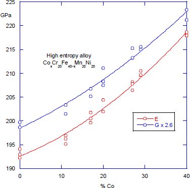
Figure 8.3. Evolution with temperature of Young’s and shear moduli for a high-entropy alloy. For a color version of this figure, see www.iste.co.uk/gadaud/elasticity.zip
The second example refers to sintered porous silver in massive form already studied in Chapter 5 (section 5.4.1). Figure 8.3 shows the evolution of the shear modulus with the porosity fraction. The correlation is still excellent, and under the hypothesis of isotropy (E/G=2(1+ν)), it allows the application of the Ramakrishnan model (Ramakrishnan and Arunachalam 1990) using relations [5.11] and [5.12]. Figure 8.3 shows that this approach also reproduces at best the experimental measurements of the shear modulus.

Figure 8.4. Evolution with temperature of Young’s and shear moduli of porous bulk silver (Caccuri et al. 2014)
8.4. Torsion of composite plate
Consider a composite plate of length L and width H; it is composed of a substrate (thickness B, density ρs and shear modulus Gs) and a coating (thickness b, density ρd and shear modulus Gd). Given the complexity of the Lagrangian approach in this configuration, only the case b<<B is considered and only the displacement of the neutral fiber is taken into account, making the hypothesis that in this case a first-order expansion in b/B is sufficient, similar to the bending case (equation [7.41]).
The local relations giving displacement and deformation are identical to expressions from equations [8.10]–[8.14]. The deformation and displacement energies are written as:
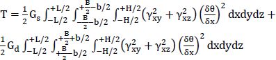

These expressions can be written more explicitly as follows:

The function f(y) is identified similarly to the homogeneous plate, which yields:
The last stage of the calculation involves the integration with respect to y of the Lagrangian expression and its simplification considering B<<H, which yields:

The minimization is done similarly to the homogeneous plate. and finally, the frequency variation introduced by the coating (first order approximation) is written as:
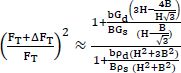
This new relation can be used to characterize the shear modulus of coatings by a differential measure between the uncoated and coated plate; however, it is currently a case study, as no experimental application was conducted.
The users who require elasticity data on coatings make do with Young’s modulus and deduce the shear modulus from Poisson’s ratio (often of the equivalent bulk material) estimated in the hypothesis of coating anisotropy. This remains a significant source of error.