
7
Beam Bending
7.1. Homogeneous beam bending without shear
Consider a homogeneous beam of length L along x, thickness B along z, modulus E and density ρ subjected to bending. With the usual notations, u is the displacement along x and w along z. According to the Euler–Bernoulli kinematic hypothesis (zero shear γxz), the following can be written as:
Since the displacement w does not depend on z, integration with respect to z yields:
The only existing deformation is longitudinal along x, which can be written as:
Denoting by FF the bending resonance frequency, the deformation and displacement energies are:

The rotational kinetic energy is negligible compared to the translational energy according to the hypothesis of no deformation under shear force and therefore no shear. The expressions of the Lagrangian and its minimization are:
A first integration by parts yields a first boundary condition and a new expression of the minimization:
A second integration by parts yields a second boundary condition and the equation of vibration:
The particular boundary conditions correspond to zero bending moment and zero shear force. These conditions are valid only for the free vibration mode; when specific conditions such as clamp are imposed, other sets of two null nth-order derivatives replace [7.8] and [7.10] (0 ≤ n ≤ 3).
The solution to the differential equation [7.11] in the case of the fundamental mode, which is symmetric with respect to x, can be written as:
Therefore, the values of two constants must be found: C and λ, the eigenvalue of the equation of vibration. The resolution of the vibration equation yields:
The two boundary conditions lead to the following system of equations:
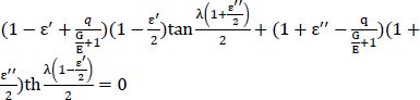
If C is eliminated by a linear combination of the two equations, then λ verifies the following:
For the fundamental mode, λ = 4.73. Inserting this value into equation [7.13] yields exactly equation [5.1] with T = 1.
Moreover, the vibration nodes (w = 0) are at 0.224 and 0.776 of the sample length; the sample length on the measurement head must meet these conditions in order to be in unperturbed free vibration mode.
7.2. Homogeneous beam bending with shear
7.2.1. Homogeneous beam bending with shear (rotation)
Despite a small B/L ratio, there is however a low-amplitude shear component that should be taken into account. It can be considered that either the displacement u is not actually proportional to z or that there is a slight variation of the section rotation. This problem is addressed using the second hypothesis as follows:
This makes it possible to express shear using the function ψ, which is unknown:
The deformation and displacement energies become:
The Lagrangian can be deduced from the above, and the minimization by integration by parts is conducted in two steps, considering w and ψ separately. Let us first consider ψ; the boundary conditions and the general equation are:
As far as w is concerned, there is also a boundary condition and a general condition:
Differentiating [7.22] with respect to x and inserting the result in [7.24] in order to eliminate ψ and keeping only the corrective terms of first order (the second-order terms in (2πFF)4 are neglected), the vibration equation and the boundary conditions are obtained:
Resuming the definition of λ (equation [7.13]), these three equations can be rewritten as follows:
The new solution to the differential equation [7.28] for the fundamental mode, which is symmetric in x, can be written as:
The system to be solved is then:
The linear combination of [7.32] and [7.33] yields:
The linear combination of [7.34] and [7.35] yields:

Considering the corrective term q, which is infinitesimal:
The two previous relations can be written as:
It should be noted that the new eigenvalues λ’ and λ’’ are very close to λ and that relation [7.40] is a more complex formulation of relation [7.16]. The eigenvalues can be rewritten as:
ε’ and ε’’ are corrective terms of first order in (B/L)2. Equations [7.39] and [7.40] yield a new system of equations:
The first-order expansion leads to two new formulations:
The two corrective terms can therefore be deduced by linear combination:
Resuming the corrective factor T introduced by the shear (equation [5.1]), it can be written as:

7.2.2. Homogeneous beam bending with shear (deformation)
For the thicker beams, it is well known that the transverse section is deformed during bending, which proves that shear should be introduced in a more realistic manner than in the previous section. The deformation energy can be rewritten taking into account only the u and w displacements:
Minimizing the deformation energy yields:

This can be solved separately for the two unknown functions u and w. Let us start by w: the boundary condition in z = ±B/2 and the general equation are, respectively:
As far as u is concerned, the boundary conditions in x = ±L/2, z = ±B/2 and the general equation are, respectively:
Equation [7.53] is integrated with respect to z and differentiated with respect to x, which yields:
Integrating this latter relation into equation [7.56], the following new relation is obtained:
Integrating a first time with respect to z and using the boundary condition [7.54], the following expression is obtained:
A second integration with respect to z yields the expression of longitudinal displacement:
Finally, the two deformations are:
The first expression shows that the longitudinal deformation is slightly affected by the shear effect.
The second one is very satisfactory, as it gives a parabolic dependence of shear with z and proportional to the shear force in x. The Lagrangian can then be rewritten as follows:

After integration with respect to z, a new one-dimensional expression of the Lagrangian is obtained (the sign ≈ is used because the term in 1/10 is not quite exact):

In order to minimize this Lagrangian, a new function p is defined to make the writing less burdensome:

The energy is once again minimized by working separately on the two functions w and p. First of all for p, the boundary condition and the general equation are, respectively:
Then, for w, the boundary condition and the general equation are:
If relation [7.68] is differentiated with respect to x and relation [7.70] is inserted into it, the general equation of vibration is obtained:
The two boundary conditions in L/2 resulting from relations [7.67] and [7.69] become:
The displacement has the same form as in equation [7.31] with two eigenvalues λ’ and λ’’ and the new system to be solved is therefore:
A linear combination of [7.73] and [7.74] yields:
Moreover, a linear combination of [7.75] and [7.76] yields:
Considering the corrective term q’, which is an infinitesimal:
The two previous relations can be written as:
As previously, λ’ and λ’’, the eigenvalues of the vibration equation are very close to λ and relation [7.81] is a more complex formulation of relation [7.16]. Rewriting the eigenvalues in the previous form, and introducing ε’ and ε’’ as corrective terms of first order in (B/L)2, then relation [7.39] is still verified and equation [7.81] becomes:

Using the first-order expansion leads to two new formulations:
The two corrective terms can therefore be deduced by linear combination:
Coming back to the correction factor T introduced by shearing (equation [5.1]), it can be written as:

7.2.3. Homogeneous beam bending with shear (comparison)
According to the literature (Spinner et al. 1960), the expression of the correction term is:
In order to compare the two proposed approaches to this reference, the B/L ratio was fixed at 1/20, a value that was experimentally employed. This comparison is illustrated in Figure 7.1 considering Poisson’s ratio within a realistic range.

Figure 7.1. Relative variation of the Young’s modulus measured during bending by taking into account the shear by various approaches. For a color version of this figure, see www.iste.co.uk/gadaud/elasticity.zip
It should be noted that taking shear into account has very little influence on the Young’s modulus for the geometry employed; the variation remains below 2%. The dependence on Poisson’s ratio remains also weak in the three cases. The two Lagrangian approaches give the same tendency with an excess or default error of about 0.1%. The relative error on the modulus is therefore of ± 0.1%, significantly lower than the experimental error.
As a conclusion, the Lagrangian approach considering the shear can be validated in a very satisfying manner; the use of second-order expansions may contribute to better results.
Anyway, experimental data management software uses the historical formalism.
7.3. Application to the characterization of the elasticity of bulk materials
In addition to the many illustrative cases already presented in Chapter 5, this section considers only one example taking into account a new material parameter, which is chemistry, focusing on high-entropy alloys.
These materials result from powder metallurgy by mixing five metallic components in equivalent stoichiometric amount. The proper choice of components leads to a unique disordered phase in which the five components are randomly distributed at the atomic level. Many combinations are possible, such as HfNbTaTiZr, with cc structure or CoCrFeMnNi with cfc structure. The elastic properties of these rapidly developing types of materials were already studied in collaboration with the Bochum University (Laplanche et al. 2015, Laplanche al. 2019).
It is also possible to have only three or four components, which form what is known as medium-entropy alloys, and in some cases, stoichiometry can be varied. It is the case of CoCrFeMnNi for which the proportion of Co and Fe can be varied to optimize the elastic properties. Figure 7.2 illustrates these tests, for which the experimental points were doubled or tripled. As it can be noted, there is an excellent correlation between elasticity and stoichiometry and the positive effect of adding Co to the detriment of Fe.

Figure 7.2. Elasticity of a high-entropy alloy depending on its stoichiometry
7.4. Composite beam bending (substrate + coating)
As already noted, bending tests are important for the characterization of the elasticity of structuring or functional coatings.
Consider a substrate whose properties are indexed by s and a coating of homogeneous thickness b (b<<B) whose properties are indexed by d. This section assumes that the beam is sufficiently thin, so that shear does not need to be taken into account. The presence of the coating induces a frequency shift ΔFF. The deformation and displacement energies are:

The term h appearing in the integration with respect to z is generated by the displacement of the neutral fiber due to the composite asymmetry. In order to determine it, the deformation energy must be minimized:
Solving the equation yields:
Inserting this value in [7.89] leads to the new expression of the deformation energy:
As for the displacement energy, the rotations are neglected:
The Lagrangian is written, and the energy is minimized using exactly the same method as in section 7.1 for the homogeneous beam, with a replacement of parameters in the equations as follows:
Consequently, the eigenvalue λ, the boundary conditions [7.8] and [7.10] as well as the vibration equation [7.11] are unchanged. The form of the solution is similar to [7.13] and [5.1], and the vibration equation becomes:
At the second order in b/B, the resulting equation is similar to the one given by a mechanical approach of the composite beam with equivalent bending stiffness (Pautrot and Mazot 1993):

When b/B is small, the simplified expression is:
This expression is the one given by the historical model of elasticity of thin films (Berry and Pritchet 1975). For thicker coatings, when the b/B ratio is of about 0.1 (coatings of about 150 μm thickness), the correction made between [7.99] and [7.100] is only of 1%.
A further important point concerns the coating adhesion. It must be perfect to have a perfect continuity of displacements at the interface. If this is not the case, a damage variable γ (0 ≤ γ ≤ 1) representative for this discontinuity (Wuttig and Su 1992) must be introduced:
Finally, this may seem surprising, but the most difficult task is the estimation of the coating density. For thick coatings, a differential weighing as well as the measurement of various dimensions is acceptable, but several surprises are possible; for example, in the case of NiO developed on Ni (Tatat 2012), the coating has a density of 5.2 ± 0.5 depending on the oxidation temperature, while in massive form, it is 6.7. This significant difference is due to impurities and porosity.
For thinner coatings, the differential weighing is no longer reliable and the appropriate method for estimating density should be identified.
7.5. Composite beam bending (substrate + “sandwich” coating)
This system is composed of two coatings of similar nature deposited on the reach side of the beam and having the same thickness; the interest of studying this configuration will be clarified further on. Since the problem of the neutral fiber no longer exists, the deformation energy becomes:

The displacement energy does not change, and integrating with respect to z, the expression of the Lagrangian becomes:

This is a much simpler expression than the one in the previous section. The minimization is done similarly and yields the new relation:
This gives the new relation between the frequency variation and moduli:

7.6. Application to the characterization of single coatings
The experimental determination of the Young’s modulus of the coating requires a differential measurement: first, the measurement of the substrate (equation [5.1]) and then that of the composite (equation [7.99]). The actual procedure employed is different: in fact, elaborating coatings that are homogeneous in thickness on pre-cut substrates is practically impossible, and if the deposition method adds energy (PVD, CVD, plasma torch, etc.), the elasticity of the substrate may be affected.
Therefore, the procedure involves the cutting of a uniformly coated plate and measuring first the composite. Then, an abrasive polishing is used to eliminate the coating; as it is still impossible to remove only the coating even by taking all the possible precautions, the upper part of the substrate is also removed. The frequency of the substrate is then measured, its modulus deduced and the last stage involves the recalculation of its resonance frequency with its initial thickness. As it will be seen, taking these precautions and acting rigorously contribute to obtaining reliable and reproducible experimental results.
A first illustration concerns the sintered silver studied in massive form in section 5.4.1, which is now characterized in the form of 50 μm thick coating sintered on copper and representative of the real solder. The samples were first annealed, for a reason that will be explained in Chapter 8. The density of these coatings is determined by the stereographic method (Saltykov 1958), which uses surface observations (Figure 5.15) to get to 3D porosity (Milhet 2015). Resuming the values of the modulus of the massive form and the Ramakrishnan analysis of section 5.4.1 and adding the measurements of the coatings, Figure 7.3 shows the excellent correlation of the elasticity data. Equation [7.100] was used for this example.
A further example of study is given by the Al/W system; thin samples of aluminum were coated with nanostructured tungsten films using PVD (Ben Dhia 2016). This method makes it possible to control the level of constraints in high-purity films and therefore to provide a proper densification of anisotropic tungsten with compression constraints. The result is that the density of films in this case is that of the massive material. As only the deposition of submicron films is possible, a choice was made to deposit on each side of the substrate in order to double the thicknesses of the film.

Figure 7.3. Comparison of the elasticity of porous silver under massive form or as coating (Caccuri et al. 2014). For a color version of this figure, see www.iste.co.uk/gadaud/elasticity.zip
Table 7.1. Study of the scattering of the elasticity of submicron W films
| Film thickness (nm) | ΔFF | E (GPa) |
| 200 ± 10 | 12 | 333 |
| 11 | 320 | |
| 11 | 316 | |
| 400 ± 10 | 23 | 330 |
| 23 | 325 | |
| 24 | 341 | |
| 600 ± 20 | 36 | 349 |
| 35 | 329 | |
| 35 | 331 | |
| Average | 333 ± 17 |
A systematic study of scattering on several thicknesses was conducted to verify whether the experimental limits of the method are reached. These results (equation [7.105]) are summarized in Table 7.1. The frequency variations are very weak, but the dispersion remains very reasonable. Massive tungsten having a modulus ranging between 390 and 410 GPa (Simmons and Wang 1971) raises the question of the comparison between the elasticity of nanostructured materials and that of the massive equivalent. Indeed, for each studied case, the experimental dispersion is widely variable, depending on the reproducibility of the mode of elaboration, on the density uncertainty and on the geometry defects of the coatings.
7.7. Three-layer beam bending
If the development of bending tests is related to the requirement of characterization of coatings, the latter can be simple or multi-layered. Moreover, the coating elaboration often creates a more or less thick interphase.
To address the problem by Lagrangian approach and vibration tests, the analysis is conducted similarly to that in section 7.4. Considering two adherent coatings of thicknesses b1 and b2, indexed by d1 and d2, respectively, the frequency variation related to the presence of these two coatings can be written as:
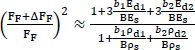
The first-order approximation is sufficient for the study of thin coatings. This formulation results from the mechanical approach of the composite beam with equivalent bending stiffness (Mazot and Pautrot 1998). The experimental procedure may vary here depending on the problem to be addressed, which will be illustrated by two examples.
Let us start by a study related to PACVD coatings of silicon carbide deposited on alloy steel. The results of the study of the Young’s modulus of the coating depending on the deposited thickness are represented in Figure 7.4, which shows a strong dependence on this parameter, even though the dispersion is here of the order of 10%.
The analysis of the interface reveals the existence of a 0.3-μm-thick interphase. The latter is not even and has a complex chemical composition involving Fe, Si and C. Considering only the most significant thicknesses, the presence of the interphase becomes negligible and the modulus extrapolated at 215 GPa corresponds to SiC, a value that is significantly lower than for the sintered massive SiC. However, for the smallest thicknesses, a three-layer system must be considered, with the presence of the interphase. Extrapolating to a zero thickness of SiC, the only one remaining is the interphase, whose density is unknown. It can be first considered very rigid, of the order of 350 GPa, if its density is equivalent to that of SiC of 3. It is more likely to consider that it is less rigid, but denser, as it contains iron.

Figure 7.4. Influence of thickness on the apparent elasticity of a SiC coating deposited on steel (Gadaud 2015)
A second illustration results from a study of the single-grained superalloy Ni-based + anticorrosive platinum aluminide (AlPtNi) + thermal barrier system that is representative for the hottest part of a turbojet engine. Figure 7.5 shows the configuration of the system; on the left, the thermal barrier (ZrO2-based) is columnar, and its thickness is of a hundred micrometers. The cutting of samples generates fragments of the surface of this fragile material; it is deposited by torch plasma after pre-oxidation. In the middle, there is a 50-μm-thick area, composed on the left of platinum aluminide (30 μm) and on the right of a 20-μm-thick interdiffusion area due to the elaboration. There is also porosity at their interface. Consequently, this two-layered film is considered as one layer whose density was estimated based on densities of superalloy, of AlPtNi and on porosity, uncertainty being recurrent. Finally, on the right, there is the single-grained superalloy oriented along <100> in the measurement direction.

Figure 7.5. Superalloy + anticorrosive platinum aluminide + thermal barrier
For this study, the superalloy substrates were covered by only one or two coatings and the experimental procedure first involved the study of the elasticity of AlPtNi as unique coating, then the one of the thermal barrier with double coating. Figure 7.6 shows the evolution of elasticity with temperature; for confidentiality reasons, the Young’s moduli are in arbitrary units. It can be seen that the evolution of the substrate is analogous to the one in Figure 6.2. The elasticity of AlPtNi first reaches a plateau and then drops sharply; this tendency is often observed when the equivalent temperature of elaboration is reached. Finally, the modulus of the thermal barrier drops rapidly. Without going into the subject, its modulus measured in the direction transverse to columns is low compared to the one of the equivalent massive material and the difference in the expansion coefficient on its metallic substrate tends to separate these columns with temperature, leading to discontinuities in terms of elasticity, as described in section 5.4.2.
Repeated tests yield a dispersion of the elasticity measurements of at least 1% for the substrate and about 5% for each coating.

Figure 7.6. Elasticity with temperature of the superalloy + anticorrosive platinum aluminide + thermal barrier (Gadaud 2015). For a color version of this figure, see www.iste.co.uk/gadaud/elasticity.zip
7.8. Multi-layered and with gradient in elastic properties of materials
The case of materials with elasticity gradient was approached for nitrided steels on a 200 μm depth in order to improve the surface properties, such as hardness (gradient of nano-precipitates from free surface to core). After treatment on a measurement sample, the sample is “peeled off” successively to relatively thin layers. For each layer indexed by i, the simplified formalism (equation [7.41]) yields:
The rate of nanoprecipitates being low, the problem of density variation is for once negligible. Eeq, Feq and deq represent, respectively, the Young’s modulus, the frequency and the thickness measured for the substrate + (i-1) layers; the thickness and the induced frequency variation are measured for each peeled-off layer. When arriving at a depth for which the substrate is “healthy”, the reference of modulus Es and thickness B is obtained. For the first layer, which is the deepest one, Eeq= Es, deq = B and Feq = F. The layer-by-layer approach is reconstructed by recalculating Eeq and Feq (deq is measured) for the substrate + (i-1) layers system.
These measurements are represented in Figure 7.7 for seven slices of about 30 μm. It should be noted that the dispersion is weak, but above all, that there is no increase in the modulus when getting closer to the surface, as we might expect. The rate of precipitates is too low to influence macroscopic elasticity. Anyway, this allows the validation of the method.
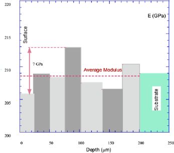
Figure 7.7. Evolution of elasticity near the surface of nitrided steel. Adapted from Gadaud (2015)
The case of multi-materials was approached through the study of friction-based brazes of titanium alloys used in aeronautics for the assembly of blades on disks. Depending on the elaboration conditions, the welding bead may have a widely variable thickness, but it is always surrounded by two different heat-affected zones (HAZ) of the two alloys in the blade and in the disk, as heat and energy are dissipated during welding.

Figure 7.8. Elasticity profile perpendicular to a welding by friction. Adapted from Gadaud (2015)
As shown in Figure 7.8, a cross-section through the welding reveals five different zones. In this case, the hypothesis is that density is approximately homogeneous, but a procedure for the study of elasticity must be found. The choice is to consider the disk or the blade as reference substrate and to cut the measurement sample at one of the edges of the welding. This is a difficult operation, which requires a first cut near the visually identifiable interface, then a series of optical observations and polishing in order to get as close as possible to the two blade (or disk) + HAZ + welding systems. The three-layer model can then be applied; the two initial titanium alloys have very close elasticity values, but the modulus tends to increase when getting near the welding.