
Despite its name, the logistic regression is a classifier. As a matter of fact, the logistic regression is one of the most commonly used discriminative learning techniques because of its simplicity and its ability to leverage a large variety of optimization algorithms. The technique is used to quantify the relationship between an observed target (or expected) variable y and a set of variables x that it depends on. Once the model is created (trained), it is available to classify real-time data.
A logistic regression can be either binomial (two classes) or multinomial (three or more classes). In a binomial classification, the observed outcome is defined as {true, false}, {0, 1}, or {-1, +1}.
The conditional probability in a linear regression model is a linear function of its weights [6:13]. The logistic regression model addresses the nonlinear regression problem by defining the logarithm of the conditional probability as a linear function of its parameters.
First, let's introduce the logistic function and its derivative, which are defined as follows (M12):
The logistic function and its derivative are illustrated in the following graph:

The graph of the logistic function and its derivative
The remainder of this section is dedicated to the application of the multivariate logistic regression to the binomial classification.
The logistic regression is popular for several reasons; some are as follows:
- It is available with most statistical software packages and open source libraries
- Its S-shape describes the combined effect of several explanatory variables
- Its range of values [0, 1] is intuitive from a probabilistic perspective
Let's consider the classification problem using two classes. As discussed in the Validation section in Chapter 2, Hello World!, even the best classifier produces false positives and false negatives. The training procedure for a binomial classification is illustrated in the following diagram:

An illustration of the binomial classification for a two-dimension dataset
The purpose of the training is to compute the hyperplane that separates the observations into two categories or classes. Mathematically speaking, a hyperplane in an n-dimensional space (number of features) is a subspace of n - 1 dimensions, as described in the Manifolds section in Chapter 4, Unsupervised Learning. The separating hyperplane of a three-dimension space is a curved surface. The separating hyperplane of a two-dimension problem (plane) is a line. In our preceding example, the hyperplane segregates/separates a training set into two very distinct classes (or groups), Class 1 and Class 2, in an attempt to reduce the overlap (false positive and false negative).
The equation of the hyperplane is defined as the logistic function of the dot product of the regression parameters (or weights) and features.
The logistic function accentuates the difference between the two groups of training observations, separated by the hyperplane. It pushes the observations away from the separating hyperplane toward either classes.
In the case of two classes, c1 and c2 with their respective probabilities, p(C=c1| X=xi|w) = p(xi|w) and p(C=c2 |X= xi|w) = 1- p(xi|w), where w is the model parameters set or weights in the case of the logistic regression.
Note
The logistic regression
M13: The log likelihood for N observations xi given regression weights w is defined as:

M14: Conditional probabilities p(x|w) with regression weights w, using the logistic function for N observations with d features {xij} j=0;d-1 is defined as:

M15: The sum of square errors, sse, for the binomial logistic regression with weights w, input values x i, and expected binary outcome y is as follows:

M16: The computation of the weights w of the logistic regression by maximizing the log likelihood, given the input data xi and expected outcome (labels) yi is defined as:

Let's implement the logistic regression without regularization using the Apache Commons Math library. The library contains several least squares optimizers that allow you to specify the optimizer minimizing algorithm for the loss function in the logistic regression class, LogisticRegression.
The constructor for the LogisticRegression class follows a very familiar pattern: it defines an ITransform data transformation, whose model is implicitly derived from the input data (training set), as described in the Monadic data transformation section in Chapter 2, Hello World! (line 2). The output of the |> predictor is a class ID, and therefore, the V type of the output is an Int (line 3):
class LogisticRegression[T <: AnyVal](
    xt: XVSeries[T],
    expected: Vector[Int],
    optimizer: LogisticRegressionOptimizer)  //1
    (implicit f: T => Double)
   extends ITransform[Array[T]](xt) with Regression
       with Monitor[Double] { //2

  type V = Int //3
    override def train: RegressionModel  //4
  def |> : PartialFunction[Array[T], Try[V]]
}
The parameters of the logistic regression class are the multivariate xt time series (features), the target or expected classes, expected, and the optimizer used to minimize the loss function or residual sum of squares (line 1). In the case of the binomial logistic regression, expected are assigned the value of 1 for one class and 0 for the other.
The Monitor trait is used to collect the profiling information during training (refer to the Monitor section under Utility classes in the Appendix A, Basic Concepts).
The purpose of the training is to determine the regression weights that minimize the loss function, as defined in the M14 formula as well as the residual sum of squares (line 4).
Note
Target values
There is no specific rule to assign the two values to the observed data for the binomial logistic regression: {-1, +1}, {0, 1}, or {false, true}. The values pair {0, 1} is convenient because it allows the developer to reuse the code for multinomial logistic regression using normalized class values.
For convenience, the definition and configuration of the optimizer are encapsulated in the LogisticRegressionOptimizer class.
The implementation of the logistic regression uses the following components:
- A
RegressionModelmodel of theModeltype that is initialized through training during the instantiation of the classifier. We reuse theRegressionModeltype, which was introduced in the Linear regression section. - The logistic regression class,
LogisticRegression, that implements anITransformfor the prediction of future observations - An adapter class named
RegressionJacobianfor the computation of the Jacobian - An adapter class named
RegressionConvergenceto manage the convergence criteria and exit condition of the minimization of the sum of square errors
The key software components of the logistic regression are described in the following UML class diagram:

The UML class diagram for the logistic regression
The UML diagram omits the helper traits or classes such as Monitor or the Apache Commons Math components.
Our implementation of the training of the logistic regression model leverages either the Gauss-Newton or the Levenberg-Marquardt nonlinear least squares optimizers, (refer to the Nonlinear least squares minimization section in the Appendix A, Basic Concepts) packaged with the Apache Commons Math library.
The training of the logistic regression is performed by the train method.
Note
Handling exceptions from the Apache Commons Math library
The training of the logistic regression using the Apache Commons Math library requires handling the ConvergenceException, DimensionMismatchException, TooManyEvaluationsException, TooManyIterationsException, and MathRuntimeException exceptions. Debugging is greatly facilitated by understanding the context of these exceptions in the Apache library source code.
The implementation of the training method, train, relies on the following five steps:
- Select and configure the least squares optimizer.
- Define the logistic function and its Jacobian.
- Specify the convergence and exit criteria.
- Compute the residuals using the least squares problem builder.
- Run the optimizer.
The workflow and the Apache Commons Math classes used in the training of the logistic regression are visualized by the following flow diagram:

The workflow for training the logistic regression using the Apache Commons Math library
The first four steps are required by the Apache Commons Math library to initialize the configuration of the logistic regression prior to the minimization of the loss function. Let's start with the configuration of the least squares optimizer:
def train: RegressionModel = {
  val weights0 = Array.fill(data.head.length +1)(INITIAL_WEIGHT)
  val lrJacobian = new RegressionJacobian(data, weights0) //5
  val exitCheck = new RegressionConvergence(optimizer) //6

  def createBuilder: LeastSquaresProblem  //7
  val optimum = optimizer.optimize(createBuilder) //8
  RegressionModel(optimum.getPoint.toArray, optimum.getRMS)
}
The train method implements the last four steps of the computation of the regression model:
- Computation of logistic values and the Jacobian matrix (line
5). - Initialization of the convergence criteria (line
6). - Definition of the least square problem (line
7). - Minimization of the sum of square errors (line
8). It is performed by the optimizer as part of the constructor ofLogisticRegression.
In this step, you have to specify the algorithm to minimize the residual of the sum of the squares. The LogisticRegressionOptimizer class is responsible for configuring the optimizer. The class has the following two purposes:
- Encapsulating the configuration parameters for the optimizer
- Invoking the
LeastSquaresOptimizerinterface defined in the Apache Commons Math library
The code will be as follows:
class LogisticRegressionOptimizer(
     maxIters: Int,
     maxEvals: Int,
     eps: Double,
     lsOptimizer: LeastSquaresOptimizer) {  //9
  def optimize(lsProblem: LeastSquaresProblem): Optimum =
       lsOptimizer.optimize(lsProblem)
}
The configuration of the logistic regression optimizer is defined as the maximum number of iterations, maxIters, the maximum number of evaluations, maxEval, for the logistic function and its derivatives, the eps convergence criteria of the residual sum of squares, and the instance of the least squares problem (line 9).
The next step consists of computing the value of the logistic function and its first order partial derivatives with respect to the weights by overriding the value method of the fitting.leastsquares.MultivariateJacobianFunction Apache Commons Math interface:
class RegressionJacobian[T <: AnyVal](  //10
    xv: XVSeries[T],
    weights0: DblArray)(implicit f: T => Double)
  extends MultivariateJacobianFunction {

  type GradientJacobian = Pair[RealVector, RealMatrix]
  override def value(w: RealVector): GradientJacobian = { //11
    val gradient = xv.map( g => { //12
      val f = logistic(dot(g, w))//13
     (f, f*(1.0-f))  //14
   })
   xv.zipWithIndex   //15
    ./:(Array.ofDim[Double](xv.size, weights0.size)) {
     case (j, (x,i)) => {
       val df = gradient(i)._2
       Range(0, x.size).foreach(n => j(i)(n+1) = x(n)*df)
       j(i)(0) = 1.0; j //16
     }
   }
   (new ArrayRealVector(gradient.map(_._1).toArray),
      new Array2DRowRealMatrix(jacobian))  //17
  }
}
The constructor for the RegressionJacobian class requires the following two arguments (line 10):
- The
xvtime series of observations - The
weights0initial regression weights
The value method uses the RealVector, RealMatrix, ArrayRealVector, and Array2DRowRealMatrix primitive types defined in the org.apache.commons.math3.linear Apache Commons Math package (line 11). It takes the w regression weight as an argument, computes the gradient (line 12) of the logistic function (line 13) for each data point, and returns the value and its derivative (line 14).
The Jacobian matrix is populated with the values of the derivative of the logistic function (line 15). The first element of each column of the Jacobian matrix is set to 1.0 to take into account the intercept (line 16). Finally, the value function returns the pair of gradient values and the Jacobian matrix using types that comply with the signature of the value method in the Apache Commons Math library (line 17).
The third step defines the exit condition for the optimizer. It is accomplished by overriding the converged method of the parameterized ConvergenceChecker interface in the org.apache.commons.math3.optim Java package:
val exitCheck = new ConvergenceChecker[PointVectorValuePair] {
  override def converged(
      iters: Int,
      prev: PointVectorValuePair,
      current:PointVectorValuePair): Boolean =
   sse(prev.getValue, current.geValue) < optimizer.eps
           && iters >= optimizer.maxIters //18
}
This implementation computes the convergence or exit condition as follows:
- The
ssesum of square errors between weights of two consecutive iterations is smaller than theepsconvergence criteria - The
itersvalue exceeds the maximum number of iterations,maxIters, allowed (line18)
The Apache Commons Math least squares optimizer package requires all the input to the nonlinear least squares minimizer to be defined as an instance of the LeastSquareProblem generated by the factory LeastSquareBuilder class:
def createBuilder: LeastSquaresProblem =
   (new LeastSquaresBuilder).model(lrJacobian)    //19
   .weight(MatrixUtils.createRealDiagonalMatrix(
             Array.fill(xt.size)(1.0)))  //20
   .target(expected.toArray) //21
   .checkerPair(exitCheck)  //22
   .maxEvaluations(optimizer.maxEvals)  //23
   .start(weights0)  //24
   .maxIterations(optimizer.maxIters) //25
   .build
The diagonal elements of the weights matrix are initialized to 1.0 (line 20). Besides the initialization of the model with the lrJacobian Jacobian matrix (line 19), the sequence of method invocations sets the maximum number of evaluations (line 23), maximum number of iterations (line 25), and the exit condition (line 22).
The regression weights are initialized with the weights0 weights as arguments of the constructor for LogisticRegression (line 24). Finally, the expected or target values are initialized (line 21).
The training is executed with a simple call to the lsp least squares minimizer:
val optimum = optimizer.optimize(lsp)
(optimum.getPoint.toArray, optimum.getRMS)
The regression coefficients (or weights) and the residuals mean square (RMS) are returned by invoking the getPoint method on the Optimum class of the Apache Commons Math library.
Let's test our implementation of the binomial multivariate logistic regression using the example of the price variation versus volatility and volume of the Copper ETF, which is used in the previous two sections. The only difference is that we need to define the target values as 0 if the ETF price decreases between two consecutive trading sessions, and 1 otherwise:
import YahooFinancials._
val maxIters = 250
val maxEvals = 4500
val eps = 1e-7

val src = DataSource(path, true, true, 1)  //26
val optimizer = new LevenbergMarquardtOptimizer  //27

for {
  price <- src.get(adjClose) //28
  volatility <- src.get(volatility)  //29
  volume <- src.get(volume)  //30
  (features, expected) <- differentialData(volatility,
volume, price, diffInt) //31
  lsOpt <- LogisticRegressionOptimizer(maxIters, maxEvals,
                        eps, optimizer) //32
  regr <- LogisticRegression[Double](features, expected, lsOpt)
  pfnRegr <- Try(regr |>) //33
}
yield {
   show(s"${LogisticRegressionEval.toString(regr)}")
   val predicted = features.map(pfnRegr(_))
   val delta = predicted.view.zip(expected.view)
            .map{case(p, e) => if(p.get == e) 1 else 0}.sum
   show(s"Accuracy: ${delta.toDouble/expected.size}")
}
Let's take a look at the steps required for the execution of the test that consists of collecting data, initializing the parameters for the minimization of the sum of square errors, training a logistic regression model, and running the prediction:
- Create a
srcdata source to extract the market and trading data (line26). - Select the
LevenbergMarquardtOptimizerLevenberg-Marquardt algorithm asoptimizer(line27). - Load the daily closing
price(line28),volatilitywithin a trading session (line29), and thevolumedaily trading (line30) for the ETF CU. - Generate the labeled data as a pair of features (the relative volatility and relative volume for the ETF) and the
expectedoutcome {0, 1} for training the model for which1represents the increase in the price and0represents the decrease in the price (line31). ThedifferentialDatageneric method of theXTSeriessingleton is described in the Time series in Scala section in Chapter 3, Data Preprocessing. - Instantiate the
lsOptoptimizer to minimize the sum of square errors during training (line32). - Train the
regrmodel and return thepfnRegrpredictor partial function (line33).
There are many alternative optimizers available to minimize the sum of square errors optimizers (refer to the Nonlinear least squares minimization section in the Appendix A, Basic Concepts).
Note
Levenberg-Marquardt parameters
The driver code uses the LevenbergMarquardtOptimizer with the default tuning parameters' configuration to keep the implementation simple. However, the algorithm has a few important parameters, such as the relative tolerance for cost and matrix inversion, that are worth tuning for commercial applications (refer to the Levenberg-Marquardt section under Nonlinear least squares minimization in the Appendix A, Basic Concepts).
The execution of the test produces the following results:
- The residual mean square is 0.497
- Weights are -0.124 for intercept, 0.453 for ETF volatility, and -0.121 for ETF volume
The last step is the classification of the real-time data.
As mentioned earlier and despite its name, the binomial logistic regression is actually a binary classifier. The classification method is implemented as an implicit data transformation |>:
val HYPERPLANE = - Math.log(1.0/INITIAL_WEIGHT -1)
def |> : PartialFunction[Array[T], Try[V]] = {
  case x: Array[T] if(isModel &&
      model.size-1 == x.length && isModel)  =>
       Try (if(dot(x, model) > HYPERPLANE) 1 else 0 ) //34
}
The dot (or inner) product of the observation x with the weights model is evaluated against the hyperplane. The predicted class is 1 if the produce exceeds HYPERPLANE, and 0 otherwise (line 34).
The direction of the price variation of the Copper ETF, CU price(t+1) – price(t), is compared to the direction predicted by the logistic regression. The result is plotted with the success value if the positive or negative direction is correctly predicted; otherwise, it is plotted with the failure value:
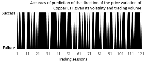
The prediction of the direction of the variation of price of the Copper ETF using the logistic regression
The logistic regression was able to classify 78 out of 121 trading sessions (65 percent accuracy).
Now, let's use the logistic regression to predict the positive price variation for the Copper ETF, given its volatility and trading volume. This trading or investment strategy is known as being long on the market. This particular use case ignores the trading sessions for which the price was either flat or declined:

The prediction of the direction of the variation of price of the Copper ETF using the logistic regression
The logistic regression was able to correctly predict the positive price variation for 58 out of 64 trading sessions (90.6 percent accuracy). What is the difference between the first and second test cases?
In the first case, the w0 + w1.volatility + w2.volume separating hyperplane equation is used to segregate the features generating either the positive or negative price variation. Therefore, the overall accuracy of the classification is negatively impacted by the overlap of the features from the two classes.
In the second case, the classifier has to consider only the observations located on the positive side of the hyperplane equation, without taking into account the false negatives.
Note
Impact of rounding errors
Under some circumstances, the generation of the rounding errors during the computation of the Jacobian matrix has an impact on the accuracy of the w0 + w1.volatility + w2.volume separating hyperplane equation. It reduces the accuracy of the prediction of both the positive and negative price variation.
The accuracy of the binary classifier can be further improved by considering the positive variation of the price using a margin error EPS as price(t+1) – price(t) > EPS.