
As the worldwide use of mobile phones has grown, a new avenue for electronic junk mail has opened for disreputable marketers. These advertisers utilize short message service (SMS) text messages to target potential consumers with unwanted advertising known as SMS spam. This type of spam is troublesome because, unlike email spam, an SMS message is particularly disruptive, due to the omnipresence of one's mobile phone. Developing a classification algorithm that could filter SMS spam would provide a useful tool for cellular phone providers.
Since Naive Bayes has been used successfully for email spam filtering, it seems likely that it could also be applied to SMS spam. However, relative to email spam, SMS spam poses additional challenges for automated filters. SMS messages are often limited to 160 characters, reducing the amount of text that can be used to identify whether a message is junk. The limit, combined with small mobile phone keyboards, has led many to adopt a form of SMS shorthand lingo, which further blurs the line between legitimate messages and spam. Let's see how a simple Naive Bayes classifier handles these challenges.
To develop the Naive Bayes classifier, we will use data adapted from the SMS Spam Collection at http://www.dt.fee.unicamp.br/~tiago/smsspamcollection/.
This dataset includes the text of SMS messages, along with a label indicating whether the message is unwanted. Junk messages are labeled spam, while legitimate messages are labeled ham. Some examples of spam and ham are shown in the following table:
|
Sample SMS ham |
Sample SMS spam |
|---|---|
|
|
Looking at the preceding messages, do you notice any distinguishing characteristics of spam? One notable characteristic is that two of the three spam messages use the word "free," yet this word does not appear in any of the ham messages. On the other hand, two of the ham messages cite specific days of the week, as compared to zero in spam messages.
Our Naive Bayes classifier will take advantage of such patterns in the word frequency to determine whether the SMS messages seem to better fit the profile of spam or ham. While it's not inconceivable that the word "free" would appear outside of a spam SMS, a legitimate message is likely to provide additional words giving context. For instance, a ham message might ask, "Are you free on Sunday?" whereas a spam message might use the phrase "free ringtones." The classifier will compute the probability of spam and ham given the evidence provided by all the words in the message.
The first step towards constructing our classifier involves processing the raw data for analysis. Text data is challenging to prepare because it is necessary to transform the words and sentences into a form that a computer can understand. We will transform our data into a representation known as bag-of-words, which ignores word order and simply provides a variable indicating whether the word appears at all.
We'll begin by importing the CSV data and saving it to a data frame:
> sms_raw <- read.csv("sms_spam.csv", stringsAsFactors = FALSE)
Using the str() function, we see that the sms_raw data frame includes 5,559 total SMS messages with two features: type and text. The SMS type has been coded as either ham or spam. The text element stores the full raw SMS message text.
> str(sms_raw)
'data.frame':    5559 obs. of  2 variables:
 $ type: chr  "ham" "ham" "ham" "spam" ...
 $ text: chr  "Hope you are having a good week. Just checking in" "K..give back my thanks." "Am also doing in cbe only. But have to pay." "complimentary 4 STAR Ibiza Holiday or £10,000 cash needs your URGENT collection. 09066364349 NOW from Landline not to lose out"| __truncated__ ...
The type element is currently a character vector. Since this is a categorical variable, it would be better to convert it to a factor, as shown in the following code:
> sms_raw$type <- factor(sms_raw$type)
Examining this with the str() and table() functions, we see that type has now been appropriately recoded as a factor. Additionally, we see that 747 (about 13 percent) of SMS messages in our data were labeled as spam, while the others were labeled as ham:
> str(sms_raw$type)
 Factor w/ 2 levels "ham","spam": 1 1 1 2 2 1 1 1 2 1 ...
> table(sms_raw$type)
 ham spam
4812  747
For now, we will leave the message text alone. As you will learn in the next section, processing the raw SMS messages will require the use of a new set of powerful tools designed specifically to process text data.
SMS messages are strings of text composed of words, spaces, numbers, and punctuation. Handling this type of complex data takes a large amount of thought and effort. One needs to consider how to remove numbers and punctuation; handle uninteresting words, such as and, but, and or; and how to break apart sentences into individual words. Thankfully, this functionality has been provided by members of the R community in a text mining package titled tm.
The tm package can be installed via the install.packages("tm") command and loaded with the library(tm) command. Even if you already have it installed, it may be worth re-running the install command to ensure that your version is up-to-date, as the tm package is still under active development. This occasionally results in changes to its functionality.
Tip
This chapter was tested using tm version 0.7-6, which was current as of February 2019. If you see differences in the output or if the code does not work, you may be using a different version. The Packt support page for this book, as well as its GitHub repository, will post solutions for future tm packages if significant changes are noted.
The first step in processing text data involves creating a corpus, which is a collection of text documents. The documents can be short or long, from individual news articles, pages in a book, pages from the web, or even entire books. In our case, the corpus will be a collection of SMS messages.
To create a corpus, we'll use the VCorpus() function in the tm package, which refers to a volatile corpus—volatile as it is stored in memory as opposed to being stored on disk (the PCorpus() function is used to access a permanent corpus stored in a database). This function requires us to specify the source of documents for the corpus, which could be a computer's file system, a database, the web, or elsewhere.
Since we already loaded the SMS message text into R, we'll use the VectorSource() reader function to create a source object from the existing sms_raw$text vector, which can then be supplied to VCorpus() as follows:
> sms_corpus <- VCorpus(VectorSource(sms_raw$text))
The resulting corpus object is saved with the name sms_corpus.
By printing the corpus, we see that it contains documents for each of the 5,559 SMS messages in the training data:
> print(sms_corpus)
<<VCorpus>>
Metadata:  corpus specific: 0, document level (indexed): 0
Content:  documents: 5559
Now, because the tm corpus is essentially a complex list, we can use list operations to select documents in the corpus. The inspect() function shows a summary of the result. For example, the following command will view a summary of the first and second SMS messages in the corpus:
> inspect(sms_corpus[1:2])
<<VCorpus>>
Metadata:  corpus specific: 0, document level (indexed): 0
Content:  documents: 2

[[1]]
<<PlainTextDocument>>
Metadata:  7
Content:  chars: 49

[[2]]
<<PlainTextDocument>>
Metadata:  7
Content:  chars: 23
To view the actual message text, the as.character() function must be applied to the desired messages. To view one message, use the as.character() function on a single list element, noting that the double-bracket notation is required:
> as.character(sms_corpus[[1]])
[1] "Hope you are having a good week. Just checking in"
To view multiple documents, we'll need to apply as.character() to several items in the sms_corpus object. For this, we'll use the lapply() function, which is part of a family of R functions that applies a procedure to each element of an R data structure. These functions, which include apply() and sapply()among others, are one of the key idioms of the R language. Experienced R coders use these much like the way for or while loops are used in other programming languages, as they result in more readable (and sometimes more efficient) code. The lapply() function for applying as.character() to a subset of corpus elements is as follows:
> lapply(sms_corpus[1:2], as.character)
$'1'
[1] "Hope you are having a good week. Just checking in"

$'2'
[1] "K..give back my thanks."
As noted earlier, the corpus contains the raw text of 5,559 text messages. To perform our analysis, we need to divide these messages into individual words. First, we need to clean the text to standardize the words and remove punctuation characters that clutter the result. For example, we would like the strings Hello!, HELLO, and hello to be counted as instances of the same word.
The tm_map() function provides a method to apply a transformation (also known as a mapping) to a tm corpus. We will use this function to clean up our corpus using a series of transformations and save the result in a new object called corpus_clean.
Our first transformation will standardize the messages to use only lowercase characters. To this end, R provides a tolower() function that returns a lowercase version of text strings. In order to apply this function to the corpus, we need to use the tm wrapper function content_transformer() to treat tolower() as a transformation function that can be used to access the corpus. The full command is as follows:
> sms_corpus_clean <- tm_map(sms_corpus,
    content_transformer(tolower))
To check whether the command worked as expected, let's inspect the first message in the original corpus and compare it to the same in the transformed corpus:
> as.character(sms_corpus[[1]])
[1] "Hope you are having a good week. Just checking in"
> as.character(sms_corpus_clean[[1]])
[1] "hope you are having a good week. just checking in"
As expected, uppercase letters in the clean corpus have been replaced by lowercase versions of the same.
Let's continue our cleanup by removing numbers from the SMS messages. Although some numbers may provide useful information, the majority are likely to be unique to individual senders and thus will not provide useful patterns across all messages. With this in mind, we'll strip all numbers from the corpus as follows:
> sms_corpus_clean <- tm_map(sms_corpus_clean, removeNumbers)
Our next task is to remove filler words such as to, and, but, and or from the SMS messages. These terms are known as stop words and are typically removed prior to text mining. This is due to the fact that although they appear very frequently, they do not provide much useful information for machine learning.
Rather than define a list of stop words ourselves, we'll use the stopwords() function provided by the tm package. This function allows us to access sets of stop words from various languages. By default, common English language stop words are used. To see the default list, type stopwords() at the R command prompt. To see the other languages and options available, type ?stopwords for the documentation page.
Tip
Even within a single language, there is no single definitive list of stop words. For example, the default English list in tm includes about 174 words, while another option includes 571 words. You can even specify your own list of stop words. Regardless of the list you choose, keep in mind the goal of this transformation, which is to eliminate useless data while keeping as much useful information as possible.
The stop words alone are not a transformation. What we need is a way to remove any words that appear in the stop words list. The solution lies in the removeWords() function, which is a transformation included with the tm package. As we have done before, we'll use the tm_map() function to apply this mapping to the data, providing the stopwords() function as a parameter to indicate exactly the words we would like to remove. The full command is as follows:
> sms_corpus_clean <- tm_map(sms_corpus_clean,
    removeWords, stopwords())
Since stopwords() simply returns a vector of stop words, if we had so chosen, we could have replaced this function call with our own vector of words to remove. In this way, we could expand or reduce the list of stop words to our liking or remove a different set of words entirely.
Continuing our cleanup process, we can also eliminate any punctuation from the text messages using the built-in removePunctuation() transformation:
> sms_corpus_clean <- tm_map(sms_corpus_clean, removePunctuation)
The removePunctuation() transformation completely strips punctuation characters from the text, which can lead to unintended consequences. For example, consider what happens when it is applied as follows:
> removePunctuation("hello...world")
[1] "helloworld"
As shown, the lack of a blank space after the ellipses caused the words hello and world to be joined as a single word. While this is not a substantial problem right now, it is worth noting for the future.
Another common standardization for text data involves reducing words to their root form in a process called stemming. The stemming process takes words like learned, learning, and learns, and strips the suffix in order to transform them into the base form, learn. This allows machine learning algorithms to treat the related terms as a single concept rather than attempting to learn a pattern for each variant.
The tm package provides stemming functionality via integration with the SnowballC package. At the time of writing, SnowballC is not installed by default with tm, so do so with install.packages("SnowballC") if you have not done so already.
Note
The SnowballC package is maintained by Milan Bouchet-Valat and provides an R interface to the C-based libstemmer library, itself based on M.F. Porter's "Snowball" word stemming algorithm, a widely used open-source stemming method. For more detail, see http://snowballstem.org.
The SnowballC package provides a wordStem() function, which for a character vector, returns the same vector of terms in its root form. For example, the function correctly stems the variants of the word learn as described previously:
> library(SnowballC)
> wordStem(c("learn", "learned", "learning", "learns"))
[1] "learn"   "learn"   "learn"   "learn"
To apply the wordStem() function to an entire corpus of text documents, the tm package includes a stemDocument() transformation. We apply this to our corpus with the tm_map() function exactly as before:
> sms_corpus_clean <- tm_map(sms_corpus_clean, stemDocument)
Tip
If you receive an error message when applying the stemDocument() transformation, please confirm that you have the SnowballC package installed. With the package installed, if you encounter a message about all scheduled cores encountered errors you might also try forcing the tm_map() command to a single core by adding an additional parameter specifying mc.cores = 1.
After removing numbers, stop words, and punctuation, and also performing stemming, the text messages are left with the blank spaces that once separated the now-missing pieces. Therefore, the final step in our text cleanup process is to remove additional whitespace using the built-in stripWhitespace() transformation:
> sms_corpus_clean <- tm_map(sms_corpus_clean, stripWhitespace)
The following table shows the first three messages in the SMS corpus before and after the cleaning process. The messages have been limited to the most interesting words, and punctuation and capitalization have been removed:
|
SMS messages before cleaning |
SMS messages after cleaning |
|
> as.character(sms_corpus[1:3])

[[1]] Hope you are having a good week. Just checking in

[[2]] K..give back my thanks.[[3]] Am also doing in cbe only. But have to pay.
|
> as.character(sms_corpus_clean[1:3])

[[1]] hope good week just check

[[2]] kgive back thank[[3]] also cbe pay
|
Now that the data are processed to our liking, the final step is to split the messages into individual terms through a process called tokenization. A token is a single element of a text string; in this case, the tokens are words.
As you might assume, the tm package provides functionality to tokenize the SMS message corpus. The DocumentTermMatrix() function takes a corpus and creates a data structure called a document-term matrix (DTM) in which rows indicate documents (SMS messages) and columns indicate terms (words).
Tip
The tm package also provides a data structure for a term-document matrix (TDM), which is simply a transposed DTM in which the rows are terms and the columns are documents. Why the need for both? Sometimes it is more convenient to work with one or the other. For example, if the number of documents is small, while the word list is large, it may make sense to use a TDM because it is usually easier to display many rows than to display many columns. That said, the two are generally interchangeable.
Each cell in the matrix stores a number indicating a count of the times the word represented by the column appears in the document represented by the row. The following illustration depicts only a small portion of the DTM for the SMS corpus, as the complete matrix has 5,559 rows and over 7,000 columns:

Figure 4.8: The DTM for the SMS messages is filled with mostly zeros
The fact that each cell in the table is zero implies that none of the words listed at the top of the columns appear in any of the first five messages in the corpus. This highlights the reason why this data structure is called a sparse matrix; the vast majority of cells in the matrix are filled with zeros. Stated in real-world terms, although each message must contain at least one word, the probability of any one word appearing in a given message is small.
Creating a DTM sparse matrix from a tm corpus involves a single command:
> sms_dtm <- DocumentTermMatrix(sms_corpus_clean)
This will create an sms_dtm object that contains the tokenized corpus using the default settings, which applies minimal processing. The default settings are appropriate because we have already prepared the corpus manually.
On the other hand, if we hadn't already performed the preprocessing, we could do so here by providing a list of control parameter options to override the defaults. For example, to create a DTM directly from the raw, unprocessed SMS corpus, we can use the following command:
> sms_dtm2 <- DocumentTermMatrix(sms_corpus, control = list(
    tolower = TRUE,
    removeNumbers = TRUE,
    stopwords = TRUE,
    removePunctuation = TRUE,
    stemming = TRUE
  ))
This applies the same preprocessing steps to the SMS corpus in the same order as done earlier. However, comparing sms_dtm to the sms_dtm2, we see a slight difference in the number of terms in the matrix:
> sms_dtm
<<DocumentTermMatrix (documents: 5559, terms: 6559)>>
Non-/sparse entries: 42147/36419334
Sparsity           : 100%
Maximal term length: 40
Weighting          : term frequency (tf)

> sms_dtm2
<<DocumentTermMatrix (documents: 5559, terms: 6961)>>
Non-/sparse entries: 43221/38652978
Sparsity           : 100%
Maximal term length: 40
Weighting          : term frequency (tf)
The reason for this discrepancy has to do with a minor difference in the ordering of the preprocessing steps. The DocumentTermMatrix() function applies its cleanup functions to the text strings only after they have been split apart into words. Thus, it uses a slightly different stop words removal function. Consequently, some words are split differently than when they are cleaned before tokenization.
The differences between these two cases illustrate an important principle of cleaning text data: the order of operations matters. With this in mind, it is very important to think through how early steps in the process are going to affect later ones. The order presented here will work in many cases, but when the process is tailored more carefully to specific datasets and use cases, it may require rethinking. For example, if there are certain terms you hope to exclude from the matrix, consider whether to search for them before or after stemming. Also consider how the removal of punctuation—and whether the punctuation is eliminated or replaced by blank space—affects these steps.
With our data prepared for analysis, we now need to split the data into training and test datasets, so that after our spam classifier is built, it can be evaluated on data it had not previously seen. However, even though we need to keep the classifier blinded as to the contents of the test dataset, it is important that the split occurs after the data have been cleaned and processed. We need exactly the same preparation steps to have occurred on both the training and test datasets.
We'll divide the data into two portions: 75 percent for training and 25 percent for testing. Since the SMS messages are sorted in a random order, we can simply take the first 4,169 for training and leave the remaining 1,390 for testing. Thankfully, the DTM object acts very much like a data frame and can be split using the standard [row, col] operations. As our DTM stores SMS messages as rows and words as columns, we must request a specific range of rows and all columns for each:
> sms_dtm_train <- sms_dtm[1:4169, ]
> sms_dtm_test  <- sms_dtm[4170:5559, ]
For convenience later on, it is also helpful to save a pair of vectors with the labels for each of the rows in the training and testing matrices. These labels are not stored in the DTM, so we need to pull them from the original sms_raw data frame:
> sms_train_labels <- sms_raw[1:4169, ]$type
> sms_test_labels  <- sms_raw[4170:5559, ]$type
To confirm that the subsets are representative of the complete set of SMS data, let's compare the proportion of spam in the training and test data frames:
> prop.table(table(sms_train_labels))
      ham      spam
0.8647158 0.1352842
> prop.table(table(sms_test_labels))
      ham      spam
0.8683453 0.1316547
Both the training data and test data contain about 13 percent spam. This suggests that the spam messages were divided evenly between the two datasets.
A word cloud is a way to visually depict the frequency at which words appear in text data. The cloud is composed of words scattered somewhat randomly around the figure. Words appearing more often in the text are shown in a larger font, while less common terms are shown in smaller fonts. This type of figure grew in popularity as a way to observe trending topics on social media websites.
The wordcloud package provides a simple R function to create this type of diagram. We'll use it to visualize the words in SMS messages. Comparing the clouds for spam and ham messages will help us gauge whether our Naive Bayes spam filter is likely to be successful. If you haven't already done so, install and load the package by typing install.packages("wordcloud") and library(wordcloud) at the R command-line.
Note
The wordcloud package was written by Ian Fellows. For more information about this package, visit his blog at: http://blog.fellstat.com/?cat=11.
A word cloud can be created directly from a tm corpus object using the syntax:
> wordcloud(sms_corpus_clean, min.freq = 50, random.order = FALSE)
This will create a word cloud from our prepared SMS corpus. Since we specified random.order = FALSE, the cloud will be arranged in non-random order, with higher-frequency words placed closer to the center. If we do not specify random.order, the cloud will be arranged randomly by default.
The min.freq parameter specifies the number of times a word must appear in the corpus before it will be displayed in the cloud. Since a frequency of 50 is about one percent of the corpus, this means that a word must be found in at least one percent of the SMS messages to be included in the cloud.
The resulting word cloud should appear similar to the following:
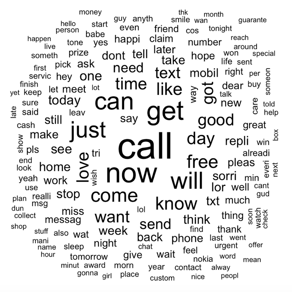
Figure 4.9: A word cloud depicting words appearing in all SMS messages
A perhaps more interesting visualization involves comparing the clouds for SMS spam and ham. Since we did not construct separate corpora for spam and ham, this is an appropriate time to note a very helpful feature of the wordcloud() function. Given a vector of raw text strings, it will automatically apply common text preparation processes before displaying the cloud.
Let's use R's subset() function to take a subset of the sms_raw data by the SMS type. First, we'll create a subset where the type is spam:
> spam <- subset(sms_raw, type == "spam")
Next, we'll do the same thing for the ham subset:
> ham <- subset(sms_raw, type == "ham")
We now have two data frames, spam and ham, each with a text feature containing the raw text strings for SMS messages. Creating word clouds is as simple as before. This time, we'll use the max.words parameter to look at the 40 most common words in each of the two sets. The scale parameter allows us to adjust the maximum and minimum font size for words in the cloud. Feel free to adjust these parameters as you see fit. This is illustrated in the following code:
> wordcloud(spam$text, max.words = 40, scale = c(3, 0.5))
> wordcloud(ham$text, max.words = 40, scale = c(3, 0.5))
The resulting word clouds should appear similar to the following:

Figure 4.10: Side-by-side word clouds depicting SMS spam and ham messages
Do you have a hunch which one is the spam cloud and which represents ham?
As you probably guessed, the spam cloud is on the left. Spam messages include words such as urgent, free, mobile, claim, and stop; these terms do not appear in the ham cloud at all. Instead, ham messages use words such as can, sorry, need, and time. These stark differences suggest that our Naive Bayes model will have some strong key words to differentiate between the classes.
The final step in the data preparation process is to transform the sparse matrix into a data structure that can be used to train a Naive Bayes classifier. Currently, the sparse matrix includes over 6,500 features; this is a feature for every word that appears in at least one SMS message. It's unlikely that all of these are useful for classification. To reduce the number of features, we'll eliminate any word that appears in less than five messages, or in less than about 0.1 percent of records in the training data.
Finding frequent words requires the use of the findFreqTerms() function in the tm package. This function takes a DTM and returns a character vector containing the words that appear at least a minimum number of times. For instance, the following command displays the words appearing at least five times in the sms_dtm_train matrix:
> findFreqTerms(sms_dtm_train, 5)
The result of the function is a character vector, so let's save our frequent words for later:
> sms_freq_words <- findFreqTerms(sms_dtm_train, 5)
A peek into the contents of the vector shows us that there are 1,139 terms appearing in at least five SMS messages:
> str(sms_freq_words)
 chr [1:1139] "£wk" "€˜m" "€˜s" "abiola" "abl" "abt" "accept" "access" "account" "across" "act" "activ" ...
We now need to filter our DTM to include only the terms appearing in the frequent word vector. As before, we'll use data frame style [row, col] operations to request specific sections of the DTM, noting that the columns are named after the words the DTM contains. We can take advantage of this fact to limit the DTM to specific words. Since we want all rows but only the columns representing the words in the sms_freq_words vector, our commands are:
> sms_dtm_freq_train <- sms_dtm_train[ , sms_freq_words]
> sms_dtm_freq_test <- sms_dtm_test[ , sms_freq_words]
The training and test datasets now include 1,139 features, which correspond to words appearing in at least five messages.
The Naive Bayes classifier is usually trained on data with categorical features. This poses a problem, since the cells in the sparse matrix are numeric and measure the number of times a word appears in a message. We need to change this to a categorical variable that simply indicates yes or no, depending on whether the word appears at all.
The following defines a convert_counts() function to convert counts to Yes or No strings:
> convert_counts <- function(x) {
    x <- ifelse(x > 0, "Yes", "No")
  }
By now, some of the pieces of the preceding function should look familiar. The first line defines the function. The statement ifelse(x > 0, "Yes", "No") transforms the values in x such that if the value is greater than 0, then it will be replaced with "Yes", otherwise it will be replaced by a "No" string. Lastly, the newly transformed vector x is returned.
We now need to apply convert_counts() to each of the columns in our sparse matrix. You may be able to guess the R function to do exactly this. The function is simply called apply() and is used much like lapply() was used previously.
The apply() function allows a function to be used on each of the rows or columns in a matrix. It uses a MARGIN parameter to specify either rows or columns. Here, we'll use MARGIN = 2 since we're interested in the columns (MARGIN = 1 is used for rows). The commands to convert the training and test matrices are as follows:
> sms_train <- apply(sms_dtm_freq_train, MARGIN = 2,
    convert_counts)
> sms_test  <- apply(sms_dtm_freq_test, MARGIN = 2,
    convert_counts)
The result will be two character-type matrices, each with cells indicating "Yes" or "No" for whether the word represented by the column appears at any point in the message represented by the row.
Now that we have transformed the raw SMS messages into a format that can be represented by a statistical model, it is time to apply the Naive Bayes algorithm. The algorithm will use the presence or absence of words to estimate the probability that a given SMS message is spam.
The Naive Bayes implementation we will employ is in the e1071 package. This package was developed at the statistics department at the Vienna University of Technology (TU Wien) and includes a variety of functions for machine learning. If you have not done so already, be sure to install and load the package using the install.packages("e1071") and library(e1071) commands before continuing.
Unlike the k-NN algorithm we used for classification in the previous chapter, training a Naive Bayes learner and using it for classification occur in separate stages. Still, as shown in the following table, these steps are fairly straightforward:
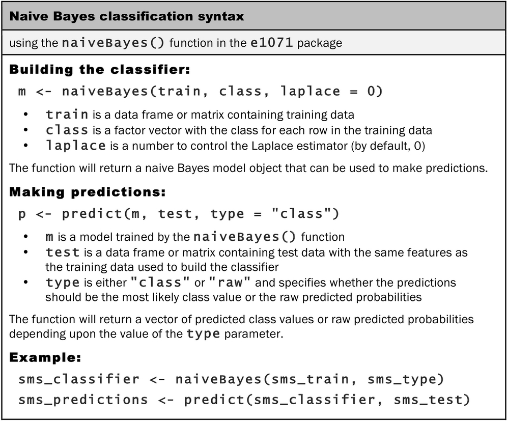
To build our model on the sms_train matrix, we'll use the following command:
> sms_classifier <- naiveBayes(sms_train, sms_train_labels)
The sms_classifier variable now contains a naiveBayes classifier object that can be used to make predictions.
To evaluate the SMS classifier, we need to test its predictions on the unseen messages in the test data. Recall that the unseen message features are stored in a matrix named sms_test, while the class labels (spam or ham) are stored in a vector named sms_test_labels. The classifier that we trained has been named sms_classifier. We will use this classifier to generate predictions and then compare the predicted values to the true values.
The predict() function is used to make the predictions. We will store these in a vector named sms_test_pred. We simply supply this function with the names of our classifier and test dataset as shown:
> sms_test_pred <- predict(sms_classifier, sms_test)
To compare the predictions to the true values, we'll use the CrossTable() function in the gmodels package, which we used previously. This time, we'll add some additional parameters to eliminate unnecessary cell proportions, and use the dnn parameter (dimension names) to relabel the rows and columns as shown in the following code:
> library(gmodels)
> CrossTable(sms_test_pred, sms_test_labels,
    prop.chisq = FALSE, prop.c = FALSE, prop.r = FALSE,
    dnn = c('predicted', 'actual'))
This produces the following table:
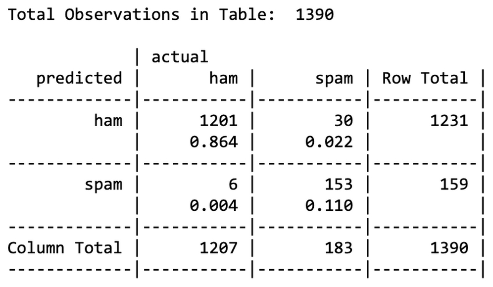
Looking at the table, we can see that a total of only 6 + 30 = 36 of 1,390 SMS messages were incorrectly classified (2.6 percent). Among the errors were six out of 1,207 ham messages that were misidentified as spam, and 30 of 183 spam messages that were incorrectly labeled as ham. Considering the little effort that we put into the project, this level of performance seems quite impressive. This case study exemplifies the reason why Naive Bayes is so often used for text classification: directly out of the box, it performs surprisingly well.
On the other hand, the six legitimate messages that were incorrectly classified as spam could cause significant problems for the deployment of our filtering algorithm, because the filter could cause a person to miss an important text message. We should investigate to see whether we can slightly tweak the model to achieve better performance.
You may have noticed that we didn't set a value for the Laplace estimator when training our model. This allows words that appeared in zero spam or zero ham messages to have an indisputable say in the classification process. Just because the word "ringtone" only appeared in spam messages in the training data, it does not mean that every message with this word should be classified as spam.
We'll build a Naive Bayes model as before, but this time set laplace = 1:
> sms_classifier2 <- naiveBayes(sms_train, sms_train_labels,
    laplace = 1)
Next, we'll make predictions:
> sms_test_pred2 <- predict(sms_classifier2, sms_test)
Finally, we'll compare the predicted classes to the actual classifications using a cross tabulation:
> CrossTable(sms_test_pred2, sms_test_labels,
    prop.chisq = FALSE, prop.c = FALSE, prop.r = FALSE,
    dnn = c('predicted', 'actual'))
This results in the following table:
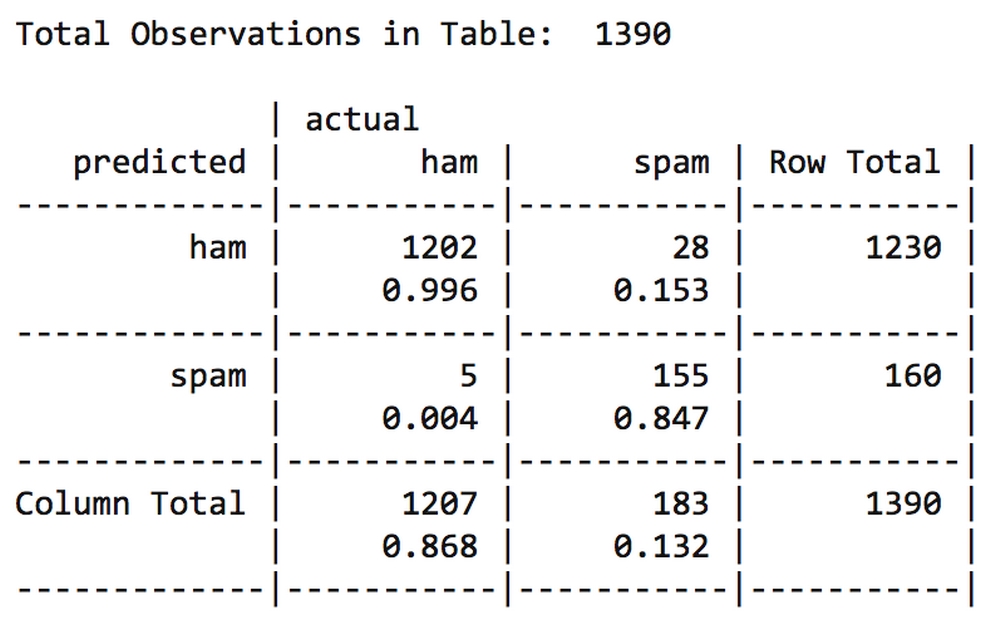
Adding the Laplace estimator reduced the number of false positives (ham messages erroneously classified as spam) from six to five, and the number of false negatives from 30 to 28. Although this seems like a small change, it's substantial considering that the model's accuracy was already quite impressive. We'd need to be careful before tweaking the model too much more, as it is important to maintain a balance between being overly aggressive and overly passive when filtering spam. Users would prefer that a small number of spam messages slip through the filter rather than an alternative in which ham messages are filtered too aggressively.