The tidyverse collection includes the tibble package and data structure—named as a pun on the word "table." A tibble acts almost exactly like a data frame but includes additional functionality for convenience and simplicity. They can be used almost everywhere a data frame can be used. Detailed information about tibbles can be found in the corresponding R for Data Science chapter at https://r4ds.had.co.nz/tibbles.html or by typing the vignette("tibble") command in R.

Most of the time, using tibbles will be transparent and seamless. However, in case you need to convert a tibble to a data frame, use the as.data.frame() function. To go in the other direction and convert a data frame to a tibble, use the as_tibble() function as follows:

> library(tibble)
> credit <- read.csv("credit.csv")
> credit_tbl <- as_tibble(credit)

Typing the name of this object demonstrates the tibble's cleaner and more informative output than a standard data frame:

Figure 12.1: Displaying a tibble object results in more informative output than a standard data frame

It is important to note the distinctions between tibbles and data frames, as the tidyverse will automatically create a tibble object for many of its operations. Overall, you are likely to find that tibbles are less annoying than data frames. They generally make smarter assumptions about the data, which means you will spend less time redoing R's work—like recoding strings as factors or vice versa. Indeed, a key distinction between tibbles and data frames is that a tibble never assumes stringsAsFactors = TRUE. Additionally, a tibble can also use column names that would be invalid in base R, such as `my var`, as long as they are surrounded by the backtick (`) character.

Tibbles are the base object in the tidyverse and enable the additional benefits of the complementary packages outlined in the sections that follow.

The dplyr package is the heart of the tidyverse, as it provides the basic functionality that allows data to be transformed and manipulated. It also provides a straightforward way to begin working with larger datasets in R. Though there are other packages that have greater raw speed or are capable of handling even more massive datasets, dplyr is still quite capable, and is a good first step to take if you run into limitations with base R.

Combined with tidyverse tibble objects, dplyr unlocks some impressive functionality:

The dplyr grammar of working with data becomes second nature after the initial learning curve has been passed. There are five key verbs in the dplyr grammar, which perform many of the most common transformations to data tables. Beginning with a tibble, one may choose to:

These five dplyr verbs are brought together in sequences using a pipe operator. Represented by the %>% symbols, the pipe operator literally "pipes" data from one function to another. The use of pipes allows the creation of powerful chains of functions for processing tables of data.

To illustrate the power of dplyr, imagine a scenario in which you are asked to examine loan applicants 21 years old or older, and find their average loan duration (in years), grouped by whether or not the applicants defaulted. With this in mind, it is not difficult to follow the following dplyr grammar, which reads almost like a pseudocode retelling of that task:

> credit %>%
    filter(age >= 21) %>%
    mutate(years_loan_duration =
             months_loan_duration / 12) %>%
    select(default, years_loan_duration) %>%
    group_by(default) %>%
    summarize(mean_duration = mean(years_loan_duration))
# A tibble: 2 x 2
  default mean_duration
  <fct>           <dbl>
1 no               1.61
2 yes              2.09

This is just one small example of how sequences of dplyr commands can make complex data manipulation tasks simpler. This is on top of the fact that, due to dplyr's more efficient code, the steps often execute more quickly than the equivalent commands in base R! Providing a complete dplyr tutorial is beyond the scope of this book, but there are many learning resources available online, including an R for Data Science chapter at https://r4ds.had.co.nz/transform.html.

The tidyverse includes the readr package as a faster solution for loading tabular data like CSV files into R. This is described in the data import chapter in R for Data Science at https://r4ds.had.co.nz/data-import.html, but the basic functionality is simple.

The package provides a read_csv() function, much like base R's read.csv(), that loads data from CSV files. The key difference is that the tidyverse is much speedier—about 10x faster according to the package authors—and is smarter about the format of the columns to be loaded. For example, it has the capability to handle numbers with currency characters, parse date columns, and is better at handling international data.

To create a tibble from a CSV file, simply use the read_csv() function as follows:

> library(readr)
> credit <- read_csv("credit.csv")

This will use the default parsing settings, which will be displayed in the R output. The defaults may be overridden by providing the column specifications via a col() function call passed to read_csv().

What used to be a tedious and time-consuming process, requiring knowledge of specific tricks and tools across multiple R packages, has been made trivial by an R package called rio (an acronym for R input and output). This package, by Chung-hong Chan, Geoffrey CH Chan, Thomas J. Leeper, and Christopher Gandrud, is described as a "Swiss-Army Knife for Data I/O." It is capable of importing and exporting a large variety of file formats including, but not limited to, tab-separated (.tsv) and comma-separated (.csv), JSON, Stata (.dta), SPSS (.sav and .por), Microsoft Excel (.xls and .xlsx), Weka (.arff), and SAS (.sas7bdat and .xpt).

The rio package consists of three functions for working with proprietary data formats: import(), export(), and convert(). Each does exactly what you'd expect from their name. Consistent with the package's philosophy of keeping things simple, each function uses the file name extension (such as .csv or .xlsx) to guess the type of file to import, export, or convert.

For example, to import the credit data CSV file used in previous chapters, simply type:

> library(rio)
> credit <- import("credit.csv")

This creates the credit data frame as expected; as a bonus, not only did we not have to specify the CSV file type, rio automatically set stringsAsFactors = FALSE as well as other reasonable defaults.

To export the credit data frame to Microsoft Excel (.xlsx) format, use the export() function while specifying the desired filename as follows. For other formats, simply change the file extension to the desired output type.

> export(credit, "credit.xlsx")

It is also possible to convert the CSV file to another format directly, without an import step, using the convert() function. For example, this converts the credit CSV file to Stata (.dta) format:

> convert("credit.csv", "credit.dta")

Though the rio package covers many common proprietary data formats, it does not do everything. The next section covers another way to get data into R via database queries.

RStudio version 1.1 introduced a graphical approach for connecting to databases. The connections tab in the top-right portion of the interface lists all of the existing database connections found on your system. The creation of these connections is typically performed by a database administrator, and is specific to the type of database as well as the operating system. For instance, on Microsoft Windows, you may need to install the appropriate database drivers as well as use the ODBC Data Source Administrator application; on MacOS and Unix/Linux you may need to install the drivers and edit an odbc.ini file.

Complete documentation about the potential connection types and installation instructions is available at https://db.rstudio.com.

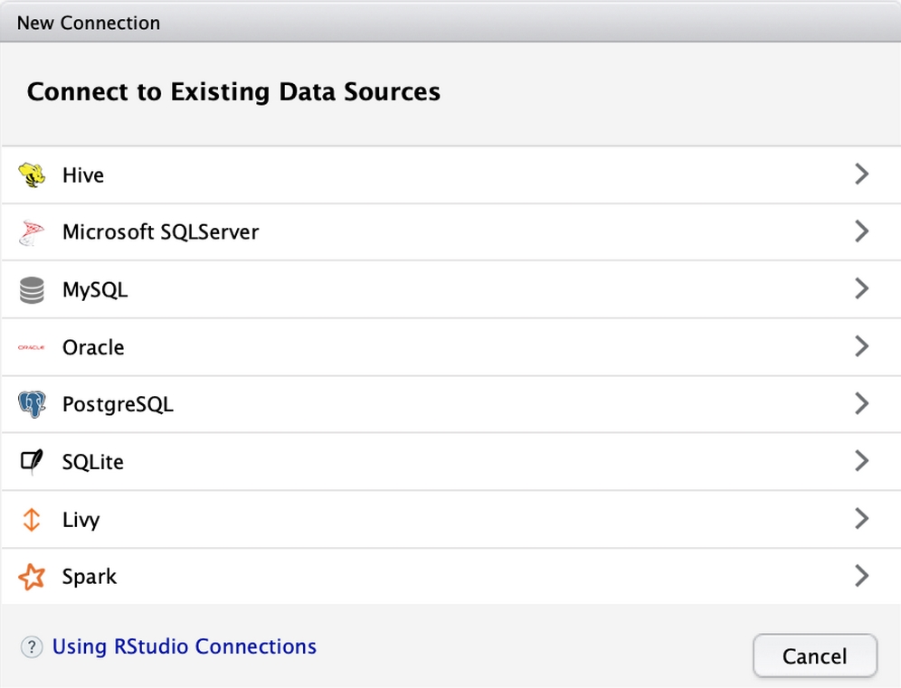
Figure 12.2: The "New Connection" button in RStudio v1.1 or greater opens an interface that will assist you with connecting to any pre-defined data sources

Behind the scenes, the graphical interface uses a variety of R packages to manage the connections to these data sources. At the core of this functionality is the DBI package, which provides a tidyverse-compliant front-end interface to the database. The DBI package also manages the back-end database driver, which must be provided by another R package. Such packages let R connect to Oracle (ROracle), MySQL (RMySQL), PostgreSQL (RPostgreSQL), and SQLite (RSQLite), among many others.

To illustrate this functionality, we'll use the DBI and RSQLite packages to connect to a SQLite database containing the credit dataset used previously. SQLite is a simple database that doesn't require running a server. It simply connects to a database file on a machine, which here is named credit.sqlite3. Before starting, be sure you've installed both of the required packages and saved the database file into your R working directory. After doing this, you can connect to the database using the following command:

> con <- dbConnect(RSQLite::SQLite(), "credit.sqlite3")

To prove the connection has succeeded, we can list the database tables to confirm the credit table exists as expected:

> dbListTables(con)
[1] "credit"

From here, we can send SQL query commands to the database and return records as R data frames. For instance, to return the loan applicants with an age of 45 years or greater, we would query the database as follows:

> res <- dbSendQuery(con, "SELECT * FROM credit WHERE age >= 45")

The entire result set can be fetched as a data frame using the following command:

> credit_age45 <- dbFetch(res)

To confirm that it worked, we'll examine the summary statistics, which confirm that the ages begin at 45 years:

> summary(credit_age45$age)
   Min. 1st Qu.  Median    Mean 3rd Qu.    Max.
  45.00   48.00   52.00   53.98   60.00   75.00

When our work is done, it is advisable to clear the query result set and close the database connection to free these resources:

> dbClearResult(res)
> dbDisconnect(con)

In addition to SQLite and the database-specific R packages, the odbc package allows R to connect to many different types of databases using a single protocol known as the Open Database Connectivity (ODBC) standard. The ODBC standard can be used regardless of operating system or DBMS.

If you have previously connected to an ODBC database, you may have referred to it via its data source name (DSN). You can use the DSN to create a database connection with a single line of R code:

> con <- dbConnect(odbc:odbc(), "my_data_source_name")

If you have a more complicated setup, or want to specify the connection properties manually, you can specify a full connection string as arguments to the DBI package dbConnect() function as follows:

> library(DBI)
> con <- dbConnect(odbc::odbc(),
                   database = "my_database",
                   uid = "my_username",
                   pwd = "my_password",
                   host = "my.server.address",
                   port = 1234)

With the connection established, queries can be sent to the ODBC database and tables can be returned as data frames using the same functions that were used for the SQLite example previously.

Connecting dplyr to an external database is no more difficult than using it with a traditional data frame. The dbplyr package (database plyr) allows any database supported by the DBI package to be used as a backend for dplyr. The connection allows tibble objects to be pulled from the database. Generally, one does not need to do more than simply install the dbplyr package, and dplyr can then take advantage of its functionality.

For example, let's connect to the SQLite credit.sqlite3 database used previously, then save its credit table as a tibble object using the tbl() function as follows:

> library(DBI)
> con <- dbConnect(RSQLite::SQLite(), "credit.sqlite3")
> credit_tbl <- con %>% tbl("credit")

In spite of the fact that dplyr has been routed through a database, the credit_tbl object here will act exactly like any other tibble and will gain all the other benefits of the dplyr package. Note that the steps would be largely similar if the SQLite database was replaced with a database residing across a network on a more traditional SQL server.

For example, to query the database for credit applicants with age at least 45 years, and display the age summary statistics for this group, we can pipe the tibble through the following sequence of functions:

> library(dplyr)
> credit_tbl %>%
    filter(age >= 45) %>%
    select(age) %>%
    collect() %>%
    summary()

      age       
 Min.   :45.00  
 1st Qu.:48.00  
 Median :52.00  
 Mean   :53.98  
 3rd Qu.:60.00  
 Max.   :75.00

Note that the dbplyr functions are "lazy," which means that no work is done in the database until it is necessary. Thus, the collect() function forces dplyr to retrieve the results from the server so that the summary statistics may be calculated.

Given a database connection, many dplyr commands will be translated seamlessly into SQL on the backend. This means that the same R code used on smaller data frames can also be used to prepare larger datasets stored in SQL databases—the heavy lifting is done on the remote server, rather than your local laptop or desktop machine. In this way, learning the tidyverse suite of packages ensures your code will apply to any type of project from small to massive.

As an alternative to the RStudio and the tidyverse approach, it is also possible to connect to SQL servers using the RODBC package by Brian Ripley. The RODBC functions retrieve data from an ODBC-compliant SQL server and create an R data frame. Although this package is still widely used, it is substantially slower in benchmarking tests than the newer odbc package, and is listed here primarily for reference.

To open a connection called mydb to the database with the DSN my_dsn, use the odbcConnect() function:

> library(RODBC)
> my_db <- odbcConnect("my_dsn")

Alternatively, if your ODBC connection requires a username and password, they should be specified when calling the odbcConnect() function:

> my_db <- odbcConnect("my_dsn",
    uid = "my_username",
    pwd = "my_password")

With an open database connection, we can use the sqlQuery() function to create an R data frame from the database rows pulled by SQL queries. This function, like many functions that create data frames, allows us to specify stringsAsFactors = FALSE to prevent R from automatically converting character data to factors.

The sqlQuery() function uses typical SQL queries as shown in the following command:

> my_query <- "select * from my_table where my_value = 1"
> results_df <- sqlQuery(channel = my_db, query = my_query,
    stringsAsFactors = FALSE)

The resulting results_df object is a data frame containing all of the rows selected using the SQL query stored in my_query.

When you are done using the database, the connection can be closed as shown in the following command:

> odbcClose(my_db)

This will close the my_db connection. Although R will automatically close ODBC connections at the end of an R session, it is better practice to do so explicitly.