
Mathematical relationships help us to make sense of many aspects of everyday life. For example, body weight is a function of one's calorie intake; income is often related to education and job experience; and poll numbers help to estimate a presidential candidate's odds of being re-elected.
When such patterns are formulated with numbers, we gain additional clarity. For example, an additional 250 kilocalories consumed daily may result in nearly a kilogram of weight gain per month; each year of job experience may be worth an additional $1,000 in yearly salary; and a president is more likely to be re-elected when the economy is strong. Obviously, these equations do not perfectly fit every situation, but we expect that they are reasonably correct most of the time.
This chapter extends our machine learning toolkit by going beyond the classification methods covered previously and introducing techniques for estimating relationships among numeric data. While examining several real-world numeric prediction tasks, you will learn:
- The basic statistical principles used in regression, a technique that models the size and strength of numeric relationships
- How to prepare data for regression analysis, and estimate and interpret a regression model
- A pair of hybrid techniques known as regression trees and model trees, which adapt decision tree classifiers for numeric prediction tasks
Based on a large body of work in the field of statistics, the methods used in this chapter are a bit heavier on math than those covered previously, but don't worry! Even if your algebra skills are a bit rusty, R takes care of the heavy lifting.
Regression involves specifying the relationship between a single numeric dependent variable (the value to be predicted) and one or more numeric independent variables (the predictors). As the name implies, the dependent variable depends upon the value of the independent variable or variables. The simplest forms of regression assume that the relationship between the independent and dependent variables follows a straight line.
Note
The origin of the term "regression" to describe the process of fitting lines to data is rooted in a study of genetics by Sir Francis Galton in the late 19th century. He discovered that fathers who were extremely short or tall tended to have sons whose heights were closer to the average height. He called this phenomenon "regression to the mean."
You might recall from basic algebra that lines can be defined in a slope-intercept form similar to y = a + bx. In this form, the letter y indicates the dependent variable and x indicates the independent variable. The slope term b specifies how much the line rises for each increase in x. Positive values define lines that slope upward while negative values define lines that slope downward. The term a is known as the intercept because it specifies the point where the line crosses, or intercepts, the vertical y axis. It indicates the value of y when x = 0.

Figure 6.1: Examples of lines with various slopes and intercepts
Regression equations model data using a similar slope-intercept format. The machine's job is to identify values of a and b such that the specified line is best able to relate the supplied x values to the values of y. There may not always be a single function that perfectly relates the values, so the machine must also have some way to quantify the margin of error. We'll discuss this in depth shortly.
Regression analysis is used for a huge variety of tasks—it is almost surely the most widely used machine learning method. It can be used both for explaining the past and extrapolating into the future, and can be applied to nearly any task. Some specific use cases include:
- Examining how populations and individuals vary by their measured characteristics, in scientific studies in the fields of economics, sociology, psychology, physics, and ecology
- Quantifying the causal relationship between an event and its response, in cases such as clinical drug trials, engineering safety tests, or marketing research
- Identifying patterns that can be used to forecast future behavior given known criteria, such as for predicting insurance claims, natural disaster damage, election results, and crime rates
Regression methods are also used for statistical hypothesis testing, which determines whether a premise is likely to be true or false in light of observed data. The regression model's estimates of the strength and consistency of a relationship provide information that can be used to assess whether the observations are due to chance alone.
Regression analysis is not synonymous with a single algorithm. Rather, it is an umbrella term for a large number of methods that can be adapted to nearly any machine learning task. If you were limited to choosing only a single machine learning method to study, regression would be a good choice. One could devote an entire career to nothing else and perhaps still have much to learn.
In this chapter, we'll focus only on the most basic linear regression models—those that use straight lines. The case when there is only a single independent variable is known as simple linear regression. In the case of two or more independent variables, it is known as multiple linear regression, or simply multiple regression. Both of these techniques assume a single dependent variable that is measured on a continuous scale.
Regression can also be used for other types of dependent variables and even for some classification tasks. For instance, logistic regression is used to model a binary categorical outcome, while Poisson regression—named after the French mathematician Siméon Poisson—models integer count data. The method known as multinomial logistic regression models a categorical outcome and can therefore be used for classification. Because the same statistical principles apply across all regression methods, after understanding the linear case, learning the other variants is straightforward.
Tip
Many of the specialized regression methods fall in a class of generalized linear models (GLM). Using a GLM, linear models can be generalized to other patterns via the use of a link function, which specifies more complex forms for the relationship between x and y. This allows regression to be applied to almost any type of data.
We'll begin with the basic case of simple linear regression. Despite the name, this method is not too simple to address complex problems. In the next section, we'll see how the use of a simple linear regression model might have averted a tragic engineering disaster.
On January 28, 1986, seven crew members of the United States space shuttle Challenger were killed when a rocket booster failed, causing a catastrophic disintegration. In the aftermath, experts quickly focused on the launch temperature as a potential culprit. The rubber O-rings responsible for sealing the rocket joints had never been tested below 40° F (4° C), and the weather on launch day was unusually cold and below freezing.
With the benefit of hindsight, the accident has been a case study for the importance of data analysis and visualization. Although it is unclear what information was available to the rocket engineers and decision makers leading up to the launch, it is undeniable that better data, utilized carefully, might very well have averted this disaster.
Note
This section's analysis is based on data presented in Risk Analysis of the Space Shuttle: Pre-Challenger Prediction of Failure, Dalal SR, Fowlkes EB, and Hoadley B, Journal of the American Statistical Association, 1989, Vol. 84, pp. 945-957. For one perspective on how data may have changed the result, see Visual Explanations: Images And Quantities, Evidence And Narrative, Tufte, ER, Cheshire, CT: Graphics Press, 1997. For a counterpoint, see Representation and misrepresentation: Tufte and the Morton Thiokol engineers on the Challenger, Robison, W, Boisjoly, R, Hoeker, D, and Young, S, Science and Engineering Ethics, 2002, Vol. 8, pp. 59-81.
The rocket engineers almost certainly knew that cold temperatures could make the components more brittle and less able to seal properly, which would result in a higher chance of a dangerous fuel leak. However, given the political pressure to continue with the launch, they needed data to support this hypothesis. A regression model that demonstrated a link between temperature and O-ring failures, and could forecast the chance of failure given the expected temperature at launch, might have been very helpful.
To build the regression model, the scientists might have used the data on launch temperature and component distresses recorded during the 23 previous successful shuttle launches. A component distress indicates one of two types of problems. The first problem, called erosion, occurs when excessive heat burns up the O-ring. The second problem, called blowby, occurs when hot gasses leak through or "blow by" a poorly sealed O-ring. Since the shuttle had a total of six primary O-rings, up to six distresses could occur per flight. Though the rocket could survive one or more distress events or be destroyed with as few as one, each additional distress increased the probability of a catastrophic failure. The following scatterplot shows a plot of primary O-ring distresses detected for the previous 23 launches, as compared to the temperature at launch:

Figure 6.2: A visualization of space shuttle O-ring distresses versus launch temperature
Examining the plot, there is an apparent trend: launches occurring at higher temperatures tend to have fewer O-ring distress events. Additionally, the coldest launch (53° F) had two distress events, a level which had only been reached in one other launch. With this information in mind, the fact that the Challenger was scheduled to launch in conditions more than 20 degrees colder seems concerning. But exactly how concerned should they have been? To answer this question, we can turn to simple linear regression.
A simple linear regression model defines the relationship between a dependent variable and a single independent predictor variable using a line defined by an equation in the following form:
Aside from the Greek characters, this equation is virtually identical to the slope-intercept form described previously. The intercept, α (alpha), describes where the line crosses the y axis, while the slope, β (beta), describes the change in y given an increase of x. For the shuttle launch data, the slope would tell us the expected change in O-ring failures for each degree the launch temperature increases.
Tip
Greek characters are often used in the field of statistics to indicate variables that are parameters of a statistical function. Therefore, performing a regression analysis involves finding parameter estimates for α and β. The parameter estimates for alpha and beta are typically denoted using a and b, although you may find that some of this terminology and notation is used interchangeably.
Suppose we know that the estimated regression parameters in the equation for the shuttle launch data are a = 3.70 and b = -0.048. Consequently, the full linear equation is y = 3.70 – 0.048x. Ignoring for a moment how these numbers were obtained, we can plot the line on the scatterplot like this:
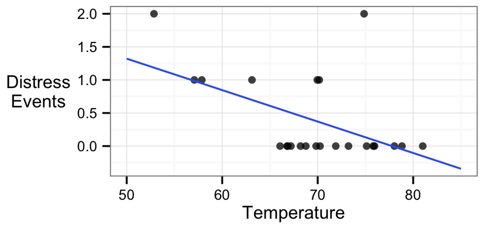
Figure 6.3: A regression line modeling the relationship between distress events and launch temperature
As the line shows, at 60 degrees Fahrenheit, we predict less than one O-ring distress. At 50 degrees Fahrenheit, we expect around 1.3 failures. If we use the model to extrapolate all the way out to 31 degrees—the forecasted temperature for the Challenger launch—we would expect about 3.70 - 0.048 * 31 = 2.21 O-ring distress events.
Assuming that each O-ring failure is equally likely to cause a catastrophic fuel leak, this means that the Challenger launch at 31 degrees was nearly three times riskier than the typical launch at 60 degrees, and over eight times riskier than a launch at 70 degrees.
Notice that the line doesn't pass through each data point exactly. Instead, it cuts through the data somewhat evenly, with some predictions lower or higher than the line. In the next section, we will learn about why this particular line was chosen.
In order to determine the optimal estimates of α and β, an estimation method known as ordinary least squares (OLS) was used. In OLS regression, the slope and intercept are chosen such that they minimize the sum of the squared errors (SSE). The errors, also known as residuals, are the vertical distance between the predicted y value and the actual y value. Because the errors can be over-estimates or under-estimates, they can be positive or negative values. These are illustrated for several points in the preceding diagram:
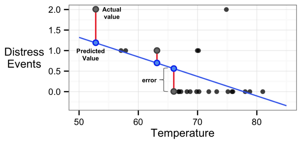
Figure 6.4: The regression line predictions differ from the actual values by a residual
In mathematical terms, the goal of OLS regression can be expressed as the task of minimizing the following equation:
In plain language, this equation defines e (the error) as the difference between the actual y value and the predicted y value. The error values are squared to eliminate the negative values and summed across all points in the data.
The solution for a depends on the value of b. It can be obtained using the following formula:
Tip
To understand these equations, you'll need to know another bit of statistical notation. The horizontal bar appearing over the x and y terms indicates the mean value of x or y. This is referred to as the x bar or y bar, and is pronounced just like the establishment you'd go to for an alcoholic drink.
Though the proof is beyond the scope of this book, it can be shown using calculus that the value of b that results in the minimum squared error is:
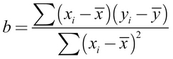
If we break this equation apart into its component pieces, we can simplify it somewhat. The denominator for b should look familiar; it is very similar to the variance of x, which is denoted as Var(x). As we learned in Chapter 2, Managing and Understanding Data, the variance involves finding the average squared deviation from the mean of x. This can be expressed as:

The numerator involves taking the sum of each data point's deviation from the mean x value multiplied by that point's deviation away from the mean y value. This is similar to the covariance function for x and y, denoted as Cov(x, y). The covariance formula is:

If we divide the covariance function by the variance function, the n terms in the numerator and denominator cancel each other and we can rewrite the formula for b as:
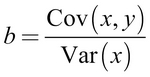
Given this restatement, it is easy to calculate the value of b using built-in R functions. Let's apply them to the shuttle launch data to estimate the regression line.
If the shuttle launch data is stored in a data frame named launch, the independent variable x is named temperature, and the dependent variable y is named distress_ct, we can then use the R functions cov() and var() to estimate b:
> b <- cov(launch$temperature, launch$distress_ct) /
         var(launch$temperature)
> b
[1] -0.04753968
We can then estimate a using the computed b value and applying the mean() function:
> a <- mean(launch$distress_ct) - b * mean(launch$temperature)
> a
[1] 3.698413
Estimating the regression equation by hand is obviously less than ideal, so R predictably provides a function for fitting regression models automatically. We will use this function shortly. Before then, it is important to expand your understanding of the regression model's fit by first learning a method for measuring the strength of a linear relationship. Additionally, you will soon learn how to apply multiple linear regression to problems with more than one independent variable.
The correlation between two variables is a number that indicates how closely their relationship follows a straight line. Without additional qualification, correlation typically refers to the Pearson correlation coefficient, which was developed by the 20th century mathematician Karl Pearson. A correlation ranges between -1 and +1. The maximum and minimum values indicate a perfectly linear relationship, while a correlation close to zero indicates the absence of a linear relationship.
The following formula defines Pearson's correlation:
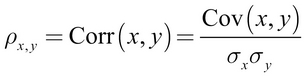
Tip
More Greek notation has been introduced here: the first symbol (which looks like a lowercase p) is rho, and it is used to denote the Pearson correlation statistic. The symbols that look like q characters rotated counter-clockwise are the Greek letter sigma, and they indicate the standard deviation of x or y.
Using this formula, we can calculate the correlation between the launch temperature and the number of O-ring distress events. Recall that the covariance function is cov() and the standard deviation function is sd(). We'll store the result in r, a letter that is commonly used to indicate the estimated correlation:
> r <- cov(launch$temperature, launch$distress_ct) /
         (sd(launch$temperature) * sd(launch$distress_ct))
> r
[1] -0.5111264
Alternatively, we can obtain the same result with the cor() correlation function:
> cor(launch$temperature, launch$distress_ct)
[1] -0.5111264
The correlation between the temperature and the number of distressed O-rings is -0.51. The negative correlation implies that increases in temperature are related to decreases in the number of distressed O-rings. To the NASA engineers studying the O-ring data, this would have been a very clear indicator that a low temperature launch could be problematic. The correlation also tells us about the relative strength of the relationship between temperature and O-ring distress. Because -0.51 is halfway to the maximum negative correlation of -1, this implies that there is a moderately strong negative linear association.
There are various rules of thumb used to interpret correlation strength. One method assigns a status of "weak" to values between 0.1 and 0.3; "moderate" to the range of 0.3 to 0.5; and "strong" to values above 0.5 (these also apply to similar ranges of negative correlations). However, these thresholds may be too strict or too lax for certain purposes. Often, the correlation must be interpreted in context. For data involving human beings, a correlation of 0.5 may be considered very high; for data generated by mechanical processes, a correlation of 0.5 may be very weak.
Tip
You have probably heard the expression "correlation does not imply causation." This is rooted in the fact that a correlation only describes the association between a pair of variables, yet there could be other unmeasured explanations. For example, there may be a strong association between life expectancy and time per day spent watching movies, but before doctors start recommending that we all watch more movies, we need to rule out another explanation: younger people watch more movies and are less likely to die.
Measuring the correlation between two variables gives us a way to quickly check for linear relationships among independent variables and the dependent variable. This will be increasingly important as we start defining regression models with a larger number of predictors.
Most real-world analyses have more than one independent variable. Therefore, it is likely that you will be using multiple linear regression for most numeric prediction tasks. The strengths and weaknesses of multiple linear regression are shown in the following table:
|
Strengths |
Weaknesses |
|---|---|
|
We can understand multiple regression as an extension of simple linear regression. The goal in both cases is similar—to find values of slope coefficients that minimize the prediction error of a linear equation. The key difference is that there are additional terms for the additional independent variables.
Multiple regression models are in the form of the following equation. The dependent variable y is specified as the sum of an intercept term α plus, for each of i features, the product of the estimated β value and the x variable. An error term ε (denoted by the Greek letter epsilon) has been added here as a reminder that the predictions are not perfect. This represents the residual term noted previously.
Let's consider for a moment the interpretation of the estimated regression parameters. You will note that in the preceding equation, a coefficient is provided for each feature. This allows each feature to have a separate estimated effect on the value of y. In other words, y changes by the amount βi for each unit increase in feature xi. The intercept α is then the expected value of y when the independent variables are all zero.
Since the intercept term α is really no different than any other regression parameter, it is also sometimes denoted as β0 (pronounced beta naught) as shown in the following equation:
Just like before, the intercept is unrelated to any of the independent x variables. However, for reasons that will become clear shortly, it helps to imagine β0 as if it were being multiplied by a term x0. We assign x0 to be a constant with the value of 1.
In order to estimate the regression parameters, each observed value of the dependent variable y must be related to observed values of the independent x variables using the regression equation in the previous form. The following figure is a graphical representation of the setup of a multiple regression task:
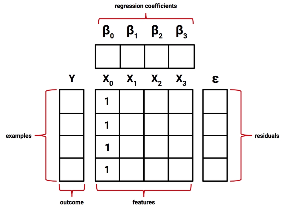
Figure 6.5: Multiple regression seeks to find the β values that relate the X values to Y while minimizing ε
The many rows and columns of data illustrated in the preceding figure can be described in a condensed formulation using matrix notation in bold font to indicate that each of the terms represents multiple values. Simplified in this way, the formula is as follows:
In matrix notation, the dependent variable is a vector, Y, with a row for every example. The independent variables have been combined into a matrix, X, with a column for each feature plus an additional column of "1" values for the intercept. Each column has a row for every example. The regression coefficients β and residual errors ε are also now vectors.
The goal now is to solve for β, the vector of regression coefficients that minimizes the sum of the squared errors between the predicted and actual Y values. Finding the optimal solution requires the use of matrix algebra; therefore, the derivation deserves more careful attention than can be provided in this text. However, if you're willing to trust the work of others, the best estimate of the vector β can be computed as:

This solution uses a pair of matrix operations: the T indicates the transpose of matrix X, while the negative exponent indicates the matrix inverse. Using R's built-in matrix operations, we can thus implement a simple multiple regression learner. Let's apply this formula to the Challenger launch data.
Tip
If you are unfamiliar with the preceding matrix operations, the Wolfram MathWorld pages for transpose (http://mathworld.wolfram.com/Transpose.html) and matrix inverse (http://mathworld.wolfram.com/MatrixInverse.html) provide a thorough introduction and are understandable even without an advanced mathematics background.
Using the following code, we can create a basic regression function named reg(), which takes a parameter y and a parameter x, and returns a vector of estimated beta coefficients:
reg <- function(y, x) {
  x <- as.matrix(x)
  x <- cbind(Intercept = 1, x)
  b <- solve(t(x) %*% x) %*% t(x) %*% y
  colnames(b) <- "estimate"
  print(b)
}
The reg() function created here uses several R commands that we have not used previously. First, since we will be using the function with sets of columns from a data frame, the as.matrix() function converts the data frame into matrix form. Next, the cbind() function binds an additional column onto the x matrix; the command Intercept = 1 instructs R to name the new column Intercept and to fill the column with repeating 1 values. Then, a series of matrix operations are performed on the x and y objects:
solve()takes the inverse of a matrixt()is used to transpose a matrix%*%multiplies two matrices
By combining these as shown, our function will return a vector b, which contains estimated parameters for the linear model relating x to y. The final two lines in the function give the b vector a name and print the result on screen.
Let's apply this function to the shuttle launch data. As shown in the following code, the dataset includes three features and the distress count (distress_ct), which is the outcome of interest:
> str(launch)
'data.frame':    23 obs. of  4 variables:
 $ distress_ct         : int  0 1 0 0 0 0 0 0 1 1 ...
 $ temperature         : int  66 70 69 68 67 72 73 70 57 63 ...
 $ field_check_pressure: int  50 50 50 50 50 50 100 100 200 ...
 $ flight_num          : int  1 2 3 4 5 6 7 8 9 10 ...
We can confirm that our function is working correctly by comparing its result for the simple linear regression model of O-ring failures versus temperature, which we found earlier to have parameters a = 3.70 and b = -0.048. Since temperature is in the second column of the launch data, we can run the reg() function as follows:
> reg(y = launch$distress_ct, x = launch[2])
               estimate
Intercept    3.69841270
temperature -0.04753968
These values exactly match our prior result, so let's use the function to build a multiple regression model. We'll apply it just as before, but this time we will specify columns two through four for the x parameter to add two additional predictors:
> reg(y = launch$distress_ct, x = launch[2:4])
                         estimate
Intercept             3.527093383
temperature          -0.051385940
field_check_pressure  0.001757009
flight_num            0.014292843
This model predicts the number of O-ring distress events using temperature, field check pressure, and the launch ID number. Notably, the inclusion of the two new predictors did not change our finding from the simple linear regression model. Just as before, the coefficient for the temperature variable is negative, which suggests that as temperature increases, the number of expected O-ring events decreases. The magnitude of the effect is also approximately the same: roughly 0.05 fewer distress events are expected for each degree increase in launch temperature.
The two new predictors also contribute to the predicted distress events. The field check pressure refers to the amount of pressure applied to the O-ring during pre-launch testing. Although the check pressure had originally been 50 psi, it was raised to 100 and 200 psi for some launches, which led some to believe that it may be responsible for O-ring erosion. The coefficient is positive, but small, providing at least a little evidence for this hypothesis. The flight number accounts for the shuttle's age. With each flight, it gets older, and parts may be more brittle or prone to fail. The small positive association between flight number and distress count may reflect this fact.
Overall, our retrospective analysis of the space shuttle data suggests that there was reason to believe that the Challenger launch was highly risky given the weather conditions. Perhaps if the engineers had applied linear regression beforehand, a disaster could have been averted. Of course, the reality of the situation, and all of the political implications involved, were surely not as simple as they appear in hindsight.
This study only scratched the surface of what is possible with linear regression modeling. Although the work was helpful for understanding exactly how regression models are built, there is more involved in modeling complex phenomena. R's built-in regression functions include additional functionality necessary to fit these more sophisticated models, and provide additional diagnostic output to aid model interpretation and assess fit. Let's apply these functions and expand our knowledge of regression by attempting a more challenging learning task.