We will use the adam (Adaptive Moment Optimization) optimizer instead of the rmsprop (Root Mean Square Propagation) optimizer that we used earlier when compiling the model. To make a comparison of model performance easier, we will keep everything else the same as earlier, as shown in the following code:

# Model architecture
model <- keras_model_sequential() %>%
         layer_embedding(input_dim = 500, output_dim = 32) %>%
         layer_lstm(units = 32) %>%
         layer_dense(units = 1, activation = "sigmoid")

# Compile
model %>% compile(optimizer = "adam",  
         loss = "binary_crossentropy",
         metrics = c("acc"))

# Fit model
model_two <- model %>% fit(train_x, train_y,
         epochs = 10,
         batch_size = 128,
         validation_split = 0.2)
plot(model_two)

After running the preceding codes and training the model, the accuracy and loss values for each epoch are stored in model_two. We use the loss and accuracy values in model_two to develop the following plot:

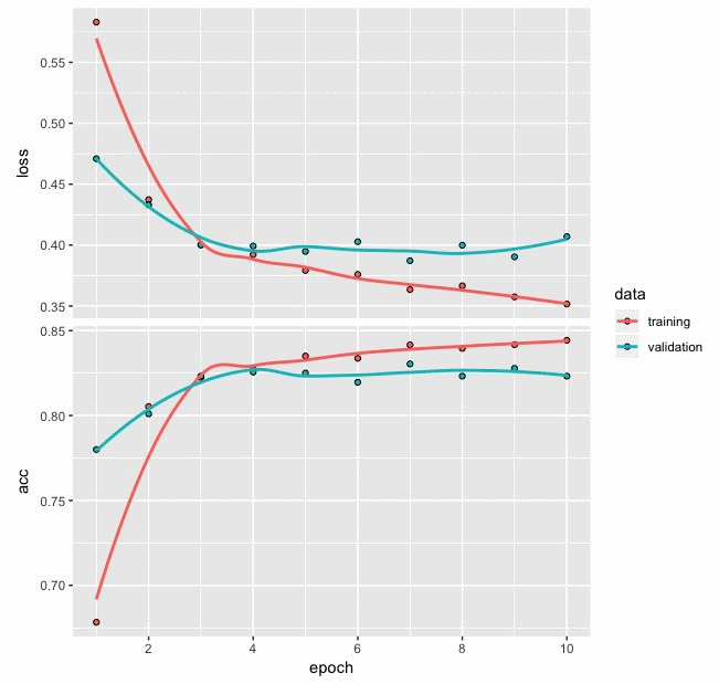
From the preceding loss and accuracy plot, we can make the following observations:

• The loss and accuracy plot based on the training and validation data shows a slightly improved pattern compared to the plot for the first model that we built with model_one.
• In the plot based on model_one, we observed that loss and accuracy values for validation data occasionally showed major deviations from the values based on the training data. In this plot, we do not see any such major deviation between the two lines.

• Also, the loss and accuracy values based on the last few values of validation data seem flat, suggesting that the ten epochs that we have used are sufficient to train the model and an increasing number of epochs is not likely to help in improving the model performance.

Next, let's obtain the loss, accuracy, and confusion matrix for the training data using the following code:

# Loss and accuracy
model %>% evaluate(train_x, train_y)
$loss
[1] 0.3601628
$acc
[1] 0.8434

pred <- model %>%   predict_classes(train_x)

# Confusion Matrix
table(Predicted=pred, Actual=imdb$train$y)
         Actual
Predicted     0     1
        0 11122  2537
        1  1378  9963

From the preceding code output, we can make the following observations:

• By using the adam optimizer, we obtain loss and accuracy for training data as 0.360 and 0.843 respectively. Both these numbers show an improvement compared to the earlier model where we had used the rmsprop optimizer.
• Another difference can be observed from the confusion matrix. This model performs better when correctly classifying negative movie reviews (at a rate of about 88.9%) compared to the correct classification of positive reviews (at a rate of about 79.7%).
• This behavior is the opposite of what was observed in the previous model. This model seems to be biased toward correctly classifying negative movie review sentiment compared to correctly classifying positive reviews.

Having reviewed the performance of the model using the training data, we will now repeat the process with the test data, with the following code for obtaining the loss, accuracy, and confusion matrix:

# Loss and accuracy
model %>% evaluate(test_x, test_y)
$loss
[1] 0.3854687
$acc
[1] 0.82868

pred1 <- model %>%   predict_classes(test_x)

# Confusion Matrix
table(Predicted=pred1, Actual=imdb$test$y)
         Actual
Predicted     0     1
        0 10870  2653
        1  1630  9847

From the preceding code output, we can make the following observations:

• The loss and accuracy based on test data are 0.385 and 0.829 respectively. These results, based on the test data, also show better model performance compared to the previous model with the test data.
• The confusion matrix shows a similar pattern that we observed for the training data. Negative movie review sentiments are correctly classified at a rate of about 86.9% for the test data.
• Similarly, positive movie review sentiments are correctly classified by the model at a rate of about 78.8% for the test data.
• This behavior is consistent with the model performance that was obtained using the training data.

Although trying the adam optimizer improves overall movie review sentiment classification performance, it still retains bias when correctly classifying one category compared to the other. A good model should not only improve the overall performance, but it should also minimize any bias when correctly classifying a category. The following code provides a table showing the number of negative and positive reviews in the train and test data:

# Number of positive and negative reviews in the train data
table(train_y)
train_y
    0     1 
12500 12500 

# Number of positive and negative review in the test data
table(test_y)
test_y
    0     1 
12500 12500 

It can be seen from the preceding output of code that this movie review data is balanced where both train and test data has 25,000 reviews each. This data is also balanced in terms of the number of positive or negative reviews. Both train and test datasets have 12,500 positive and 12,500 negative movie reviews each. Hence, there is no bias in the amount of negative or positive reviews provided to the model for training. However, the bias seen when correctly classifying negative and positive movie reviews is certainly something that needs improvement.

In the next experiment, let's explore with more LSTM layers and see whether or not we can obtain a better movie review sentiment classification model.