Search in book...
Toggle Font Controls
Create new playlist

Name your new playlist

Playlist description (optional)
Sign In

Email address

Password

Forgot Password?

or

Continue with Facebook

Continue with Google
Sign Up

Full Name

Email address

Confirm Email Address

Password

or

Continue with Facebook

Continue with Google

Reading Time Series Data from Databases

Databases extend what you can store to include text, images, and media files and are designed for efficient read and write operations at a massive scale. Databases can store terabytes and petabytes of data with efficient and optimized data retrieval capabilities, such as when we are performing analytical operations on data warehouses and data lakes. A data warehouse is a database designed to store large amounts of structured data, mostly integrated from multiple source systems, built specifically to support business intelligence reporting, dashboards, and advanced analytics. A data lake, on the other hand, stores a large amount of data that is structured, semi-structured, or unstructured in its raw format. In this chapter, we will continue to use the pandas library to read data from databases. We will create time series DataFrames by reading data from relational (SQL) databases and non-relational (NoSQL) databases.

Additionally, you will explore working with third-party data providers to pull financial data from their database systems.

In this chapter, you will create time series DataFrames with a DatetimeIndex data type by covering the following recipes:

Reading data from a relational database
Reading data from Snowflake
Reading data from a document database (MongoDB)
Reading third-party financial data using APIs
Reading data from a time series database (InfluxDB)

Technical requirements

In this chapter, we will be using pandas 1.4.2 (released April 2, 2022) extensively.

You will be working with different types of databases, such as PostgreSQL, Amazon Redshift, MongoDB, InfluxDB, and Snowflake. You will need to install additional Python libraries to connect to these databases.

You can also download the Jupyter notebooks from this book's GitHub repository (https://github.com/PacktPublishing/Time-Series-Analysis-with-Python-Cookbook) to follow along.

Reading data from a relational database

In this recipe, you will read data from PostgreSQL, a popular open source relational database.

You will explore two methods for connecting to and interacting with PostgreSQL. First, you will start by using psycopg2, a PostgreSQL Python connector, to connect and query the database, then parse the results into a pandas DataFrame. In the second approach, you will query the same database again but this time using SQLAlchemy, an object-relational mapper (ORM) that is well integrated with pandas.

Getting ready

In this recipe, it is assumed that you have the latest PostgreSQL installed. At the time of writing, version 14 is the latest stable version (version 15 is still in beta).

To connect to and query the database in Python, you will need to install psycopg2, a popular PostgreSQL database adapter for Python. You will also need to install SQLAlchemy, which provides flexibility regarding how you want to manage the database, whether it is for writing or reading data.

To install the libraries using conda, run the following command:

>>> conda install sqlalchemy psycopg2 -y

To install the libraries using pip, run the following command:

>>> pip install sqlalchemy psycopg2

How to do it…

We will start by connecting to the PostgreSQL instance, querying the database, loading the result set into memory, and finally parsing the data into a time series DataFrame.

In this recipe, I will be connecting to a PostgreSQL instance that is running locally, so my connection would be to localhost (127.0.0.1). You will need to adjust this for your own PostgreSQL database setting.

Using the psycopg2 PostgreSQL adapter for Python

psycopg2 is a Python library (and a database driver) that provides additional functionality and features when you are working with a PostgreSQL database. Follow these steps:

Start by importing the necessary libraries. Define a Python dictionary where you will store all the parameter values required to establish a connection to the database, such as host, database name, user name, and password:
```
import psycopg2
```
```
import pandas as pd
```
```
params = {
```
```
    "host": "127.0.0.1",
```
```
    "database": "postgres",
```
```
    "user": "postgres",
```
```
    "password": "password"
```
```
}
```
You can establish a connection by passing the parameters to the .connect() method. Once connected, you can create a cursor object that can be used to execute SQL queries:
```
conn = psycopg2.connect(**params)
```
```
cursor = conn.cursor()
```
The cursor object provides several attributes and methods, including execute() and fetchall(). The following code uses the cursor object to pass a SQL query and then checks the number of records that have been produced by that query using the .rowcount attribute:
```
cursor.execute("""
```
```
SELECT date, last, volume
```
```
FROM yen_tbl
```
```
ORDER BY date;
```
```
""")
```
```
cursor.rowcount
```
```
>> 10902
```
The returned result set after executing the query will not include a header (no columns names). Alternatively, you can grab the column names from the cursor object using the description attribute, as shown in the following code:
```
cursor.description
```
```
>> 
```
```
(Column(name='date', type_code=1082),
```
```
 Column(name='last', type_code=1700),
```
```
 Column(name='volume', type_code=1700))
```
You can use a list comprehension to extract the column names from cursor.description to use as column headers when creating the DataFrame:
```
columns = [col[0] for col in cursor.description]
```
```
columns
```
```
>> ['date', 'last', 'volume']
```

Now, fetch the results that were produced by the executed query and store them in a pandas DataFrame. Make sure that you pass the column names that you just captured:

data = cursor.fetchall()

df = pd.DataFrame(data, columns=columns)

df.info()

>>

<class 'pandas.core.frame.DataFrame'>

RangeIndex: 10902 entries, 0 to 10901

Data columns (total 3 columns):

 #   Column  Non-Null Count  Dtype

---  ------  --------------  -----

 0   date    10902 non-null  object

 1   last    10902 non-null  object

 2   volume  10902 non-null  object

dtypes: object(3)

memory usage: 255.6+ KB

Notice that the date column is returned as an object type, not a datetime type.

Parse the date column using pd.to_datetime() and set it as the index for the DataFrame:

df = df.set_index('date')

df.index = pd.to_datetime(df.index)

df.tail(3)

>>

            last    volume

date

2019-10-11  9267.0  158810.0

2019-10-14  9261.0  69457.0

2019-10-15  9220.0  108342.0

In the preceding code, the cursor returned a list of tuples without a header. You can instruct the cursor to return a RealDictRow type, which will include the column name information. This is more convenient when converting into a DataFrame. This can be done by passing the RealDictCursor class to the cursor_factory parameter:

from psycopg2.extras import RealDictCursor
cursor = conn.cursor(cursor_factory=RealDictCursor)
cursor.execute("SELECT * FROM yen_tbl;")
data = cursor.fetchall()
df = pd.DataFrame(data)

Close the cursor and the connection to the database:
```
In [12]: cursor.close()
```
```
In [13]: conn.close()
```

Starting from version 2.5, psycopg2 connections and cursors can be used in Python's with statement for exception handling when committing a transaction. The cursor object provides three different fetching functions; that is, fetchall(), fetchmany(), and fetchone(). The fetchone() method returns a single tuple. The following example shows this concept:

import psycopg2
url = 'postgresql://postgres:password@localhost:5432'
with psycopg2.connect(url) as conn:
     with conn.cursor() as cursor:
            cursor.execute('SELECT * FROM yen_tbl')
            data = cursor.fetchall()

Using SQLAlchemy and psycopg2

SQLAlchemy is a very popular open source library for working with relational databases in Python. SQLAlchemy can be referred to as an object-relational mapper (ORM), which provides an abstraction layer (think of an interface) so that you can use object-oriented programming to interact with a relational database.

You will be using SQLAlchemy because it integrates very well with pandas, and several of the pandas SQL reader and writer functions depend on SQLAlchemy as the abstraction layer. SQLAlchemy does the translation behind the scenes for any pandas SQL read or write requests. This translation ensures that the SQL statement from pandas is represented in the right syntax/format for the underlying database type (MySQL, Oracle, SQL Server, or PostgreSQL, to name a few).

Some of the pandas SQL reader functions that rely on SQLAlchemy include pandas.read_sql(), pandas.read_sql_query(), and pandas.read_sql_table(). Let's perform the following steps:

Start by importing the necessary libraries. Note that, behind the scenes, SQLAlchemy will use psycopg2 (or any other database driver that is installed and supported by SQLAlchemy):

import pandas as pd

from sqlalchemy import create_engine

engine = create_engine("postgresql+psycopg2://postgres:password@localhost:5432")

query = "SELECT * FROM yen_tbl"

df = pd.read_sql(query,

                 engine,

                 index_col='date',

                 parse_dates={'date': '%Y-%m-%d'})

df['last'].tail(3)

>>

date

2019-10-11    9267.0

2019-10-14    9261.0

2019-10-15    9220.0

Name: last, dtype: float64

In the preceding example, for parse_dates, you passed a dictionary in the format of {key: value}, where key is the column name and value is a string representation of the date format. Unlike the previous psycopg2 approach, pandas.read_sql() did a better job of getting the data types correct. Notice that our index is of the DatetimeIndex type:

df.info()
>>
<class 'pandas.core.frame.DataFrame'>
DatetimeIndex: 10902 entries, 1976-08-02 to 2019-10-15
Data columns (total 8 columns):
 #   Column                      Non-Null Count  Dtype  
---  ------                      --------------  -----  
 0   open                        10902 non-null  float64
 1   high                        10902 non-null  float64
 2   low                         10902 non-null  float64
 3   last                        10902 non-null  float64
 4   change                      1415 non-null   float64
 5   settle                      10902 non-null  float64
 6   volume                      10902 non-null  float64
 7   Previous Day Open Interest  10902 non-null  float64
dtypes: float64(8)
memory usage: 766.5 KB

You could also accomplish the same results using the pandas.read_sql_query() function. This will also return an index of the O type:

df = pd.read_sql_query(query,

                       engine,

                       index_col='date',

                       parse_dates={'date':'%Y-%m-%d'})

pandas provides another SQL reader function called pandas.read_sql_table() that does not take a SQL query, instead taking a table name. Think of this as a SELECT * FROM sometable query:

df = pd.read_sql_table('yen_tbl',

                        engine,

                        index_col='date')

How it works…

Let's examine the engine connection string for SQLAlchemy:

create_engine("dialect+driver://username:password@host:port/dbname")

Creating the engine is the first step when working with SQLAlchemy as it provides instructions on the database that is being considered. This is known as a dialect.

Earlier, you used psycopg2 as the database driver for PostgreSQL. psycopg2 is referred to as a database API (DBAPI) and SQLAlchemy supports many DBAPI wrappers based on Python's DBAPI specifications to connect to and interface with various types of relational databases. It also comes with built-in dialects to work with different flavors of RDBMS, such as the following:

SQL Server
SQLite
PostgreSQL
MySQL
Oracle
Snowflake

When connecting to a database using SQLAlchemy, we need to specify the dialect and the driver (DBAPI) to be used. This is what the format looks like for PostgreSQL:

create_engine("postgresql+psycopg2://username:password@localhost:5432")

In the previous code examples, we did not need to specify the psycopg2 driver since it is the default DBAPI that is used by SQLAlchemy. This example would work just fine, assuming that psycopg2 is installed:

create_engine("postgresql://username:password@localhost:5432")

There are other PostgreSQL drivers (DBAPI) that are supported by SQLAlchemy, including the following:

psycopg2
pg8000
asyncpg
pygresql

For a more comprehensive list of supported dialects and drivers, you can visit the official documentation page at https://docs.sqlalchemy.org/en/14/dialects/.

The advantage of using SQLAlchemy is that it is well integrated with pandas. If you read the official pandas documentation for read_sql(), read_sql_query(), and read_sql_table(), you will notice that the conn argument is expecting a SQLAlchemy connection object (engine).

There's more…

When you executed the query against yen_tbl, it returned 10,902 records. Imagine working with a larger database that returned millions of records, if not more. This is where chunking helps.

The chunksize parameter allows you to break down a large dataset into smaller and more manageable chunks of data that can fit into your local memory. When executing the read_sql() function, just pass the number of rows to be retrieved (per chunk) to the chunksize parameter, which then returns a generator object. You can then loop through that object or use next(), one chunksize at a time, and perform whatever calculations or processing needed. Let's look at an example of how chunking works. You will request 5 records (rows) at a time:

df = pd.read_sql(query,
                 engine,
                 index_col='date',
                 parse_dates=True,
                 chunksize=5)
# example using next 
next(df)['last']
>>
date
1976-08-02    3401.0
1976-08-03    3401.0
1976-08-04    3401.0
1976-08-05    3401.0
1976-08-06    3401.0
Name: last, dtype: float64
# example using a for loop
df = pd.read_sql(query,
                 engine,
                 index_col='date',
                 parse_dates=True,
                 chunksize=5000)
for idx, data in enumerate(df):
     print(idx, data.shape)
>>
0 (5000, 8)
1 (5000, 8)
2 (902, 8)

The preceding code demonstrated how chunking works. Using the chunksize parameter should reduce memory usage since the code loads 5,000 rows at a time. The PostgreSQL database being used contains 10,902 rows, so it took three rounds to retrieve the entire dataset: 5,000 on the first, 5,000 on the second, and the last 902 records on the third.

Reading data from Snowflake

A very common place to extract data for analytics is usually a company's data warehouse. Data warehouses host a massive amount of data that, in most cases, contains integrated data to support various reporting and analytics needs, in addition to historical data from various source systems.

The evolution of the cloud brought us cloud data warehouses such as Amazon Redshift, Google BigQuery, Azure SQL Data Warehouse, and Snowflake.

In this recipe, you will work with Snowflake, a powerful Software as a Service (SaaS) cloud-based data warehousing platform that can be hosted on different cloud platforms, such as Amazon Web Services (AWS), Google Cloud Platform (GCP), and Microsoft Azure. You will learn how to connect to Snowflake using Python to extract time series data and load it into a pandas DataFrame.

Getting ready

This recipe assumes you have access to Snowflake. To connect to Snowflake, you will need to install the Snowflake Python connector.

To install Snowflake using conda, run the following command:

conda install -c conda-forge snowflake-sqlalchemy snowflake-connector-python

To install Snowflake using pip, run the following command:

pip install "snowflake-connector-python[pandas]"
pip install --upgrade snowflake-sqlalchemy

How to do it...

We will explore two ways to connect to the Snowflake database. In the first method, you will be using the Snowflake Python connector to establish our connection, as well as to create our cursor to query and fetch the data. In the second method, you will explore SQLAlchemy and how it integrates with the pandas library. Let's get started:

We will start by importing the necessary libraries:

import pandas as pd

from snowflake import connector

from configparser import ConfigParser

The Snowflake connector has a set of input parameters that need to be supplied to establish a connector. You can create a .cfg file, such as snow.cfg, to store all the necessary information in the following format:
```
[SNOWFLAKE]
```
```
USER=<your_username>
```
```
PASSWORD=<your_password>
```
```
ACCOUNT=<your_account>
```
```
WAREHOUSE=<your_warehouse_name>
```
```
DATABASE=<your_database_name>
```
```
SCHEMA=<you_schema_name>
```
```
ROLE=<your_role_name>
```
Using ConfigParser, you can extract the content under the [SNOWFLAKE] section to avoid exposing or hardcoding your credentials. You can read the entire content of the [SNOWFLAKE] section and convert it into a dictionary object, as shown here:
```
connector.paramstyle='qmark'
```
```
config = ConfigParser()
```
```
config.read('snow.cfg')
```
```
config.sections()
```
```
params = dict(config['SNOWFLAKE'])
```
You will need to pass the parameters to connector.connect() to establish a connection with Snowflake. We can easily unpack the dictionary's content since the dictionary keys match the parameter names, as per Snowflake's documentation. Once the connection has been established, we can create our cursor:
```
con = connector.connect(**params)
```
```
cursor = con.cursor()
```
The cursor object has many methods, including execute, to pass a SQL statement to the database, as well as several fetch methods to retrieve the data. In the following example, we will query the ORDERS table and leverage the fetch_pandas_all method to get a pandas DataFrame:
```
query = "select * from ORDERS;"
```
```
cursor.execute(query)
```
```
df = cursor.fetch_pandas_all()
```

Inspect the DataFrame using df.info():

df.info()

>>

<class 'pandas.core.frame.DataFrame'>

Int64Index: 15000 entries, 0 to 4588

Data columns (total 9 columns):

 #   Column           Non-Null Count  Dtype

---  ------           --------------  -----

 0   O_ORDERKEY       15000 non-null  int32

 1   O_CUSTKEY        15000 non-null  int16

 2   O_ORDERSTATUS    15000 non-null  object

 3   O_TOTALPRICE     15000 non-null  float64

 4   O_ORDERDATE      15000 non-null  object

 5   O_ORDERPRIORITY  15000 non-null  object

 6   O_CLERK          15000 non-null  object

 7   O_SHIPPRIORITY   15000 non-null  int8

 8   O_COMMENT        15000 non-null  object

dtypes: float64(1), int16(1), int32(1), int8(1), object(5)

memory usage: 922.9+ KB

From the preceding output, you can see that the DataFrame's Index is just a sequence of numbers and that the O_ORDERDATE column is not a Date field. This can be fixed by parsing the O_ORDERDATE column with a DatetimeIndex and setting it as an index for the DataFrame:
```
df_ts = (df.set_index(pd.to_datetime(df['O_ORDERDATE']))
```
```
        .drop(columns='O_ORDERDATE'))
```
```
df_ts.iloc[0:3, 1:5]
```

Now, you should have a time series DataFrame with a DatetimeIndex (O_ORDERDATE):

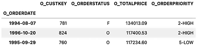
Figure 3.1 – The first three rows of the time series df_ts DataFrame

You can inspect the index of the DataFrame and print the first two indexes:

df_ts.index[0:2]

>> DatetimeIndex(['1994-08-07', '1996-10-20'], dtype='datetime64[ns]', name='O_ORDERDATE', freq=None)

The DataFrame now has O_ORDERDATE as the index and the proper data type; that is, DatetimeIndex.

You can repeat the same process but without the additional effort of manually parsing the O_ORDERDATE column and setting it as an index. Here, you can use SQLAlchemy and leverage the pandas.read_sql() reader function to perform these operations:

from sqlalchemy import create_engine

from snowflake.sqlalchemy import URL

url = URL(**params)

engine = create_engine(url)

connection = engine.connect()

df = pd.read_sql(query,

                 connection,

                 index_col='o_orderdate',

                 parse_dates='o_orderdate')

df.info()

>>

<class 'pandas.core.frame.DataFrame'>

DatetimeIndex: 15000 entries, 1994-08-07 to 1994-06-13

Data columns (total 8 columns):

 #   Column           Non-Null Count  Dtype

---  ------           --------------  -----

 0   o_orderkey       15000 non-null  int64

 1   o_custkey        15000 non-null  int64

 2   o_orderstatus    15000 non-null  object

 3   o_totalprice     15000 non-null  float64

 4   o_orderpriority  15000 non-null  object

 5   o_clerk          15000 non-null  object

 6   o_shippriority   15000 non-null  int64

 7   o_comment        15000 non-null  object

dtypes: float64(1), int64(3), object(4)

memory usage: 1.0+ MB

Notice that O_ORDERDATE is now an index and of the DatetimeIndex type.

How it works...

The Snowflake Python connector requires several input variables to connect to the database. These include the following:

Table 3.1 – Input variables for the Snowflake Python connector

For a complete list of parameters that are available for the connect() function, you can refer to the official documentation at https://docs.snowflake.com/en/user-guide/python-connector-api.html#module-snowflake-connector.

Once the connection is accepted, you could create your cursor object. The cursor provides several useful attributes and methods, including description, rowcount, rownumber, execute(), execute_async(), fetchone(), fetchall(), fetch_pandas_all(), and fetch_pandas_batches(), to name few.

For a complete list of attributes and methods, you can refer to the official documentation at https://docs.snowflake.com/en/user-guide/python-connector-api.html#object-cursor.

Using SQLAlchemy, you were able to leverage the pandas.read_sql() reader function and use the many parameters available to transform and process the data at read time. The Snowflake fetch_pandas_all() function, on the other hand, does not take in any parameters, and you will need to parse and adjust the DataFrame afterward.

The Snowflake SQLAlchemy library provides a convenience method, URL, to help construct the connection string to connect to the Snowflake database. Typically, SQLAlchemy expects a URL to be provided in the following format:

'snowflake://<user>:<password>@<account>/<database>/<schema>
?warehouse=<warehouse>&role=<role>'

Using the URL method, we passed our parameters and the method took care of constructing the connection string that is expected:

engine = create_engine(URL(
    account = '<your_account>',
    user = '<your_username>',
    password = '<your_password>',
    database = '<your_database>',
    schema = '<your_schema>',
    warehouse = '<your_warehouse>',
    role='<your_role>',
))

There's more...

You may have noticed that the columns in the returned DataFrame, when using the Snowflake Python connector, all came back in uppercase, while they were lowercased when using Snowflake SQLAlchemy.

The reason for this is because Snowflake, by default, stores unquoted object names in uppercase when these objects are created. In the previous code, for example, our Order Date column was returned as O_ORDERDATE.

To explicitly indicate the name is case-sensitive, you will need to use quotes when creating the object in Snowflake (for example, 'o_orderdate' or 'OrderDate'). In contrast, using Snowflake SQLAlchemy converts the names into lowercase by default.

Reading data from a document database (MongoDB)

MongoDB, a NoSQL database, stores data in documents and uses BSON (a JSON-like structure) to store schema-less data. Unlike relational databases, where data is stored in tables that consist of rows and columns, document-oriented databases store data in collections and documents.

A document represents the lowest granular level of data being stored, as rows do in relational databases. A collection, like a table in relational databases, stores documents. Unlike relational databases, a collection can store documents of different schemas and structures.

Getting ready

In this recipe, it is assumed that you have a running instance of MongoDB. To get ready for this recipe, you will need to install the PyMongo Python library to connect to MongoDB.

To install MongoDB using conda, run the following command:

$ conda install -c anaconda pymongo -y

To install MongoDB using pip, run the following command:

$ python -m pip install pymongo

Note about Using MongoDB Atlas

If you are connecting to MongoDB Atlas (Cloud) Free Tier or their M2/M5 shared tier cluster, then you will be using the mongodb+srv protocol. In this case, you can either specify this during the pip install with python -m pip install pymongo[srv] or you can just install dnspython with pip install dnspython.

How to do it…

In this recipe, you will connect to the MongoDB instance that you have set up. If you are using an on-premises install (local install or Docker container), then your connection string will be mongodb://localhost:27017. If you are using Atlas, then your connection may look more like mongodb+srv://<username>:<password>@<clusterName>.yqcgb.mongodb.net/<DatabaseName>?retryWrites=true&w=majority.

Perform the following steps:

First, let's import the necessary libraries:

import pandas as pd

from pymongo import MongoClient

Establish a connection to MongoDB. For a local instance (on-premises), this would look something like this:

# connecting to on-premise instance

url = "mongodb://localhost:27017"

client = MongoClient(url)

MongoClient(host=['localhost:27017'],

                 document_class=dict,

                      tz_aware=False,

                       connect=True)

>> MongoClient(host=['localhost:27017'], document_class=dict, tz_aware=False, connect=True)

If you are connecting to Atlas, the connection string will look more like this:

# connecting to Atlas cloud Cluster
cluster = 'cluster0'
username = 'user'
password = 'password'
database = 'stock_data'
url = 
f"mongodb+srv://{username}:{password}@{cluster}.3rncb.mongodb.net/{database}"
client =  MongoClient(url)
client
>> MongoClient(host=['cluster0-shard-00-00.3rncb.mongodb.net:27017', 'cluster0-shard-00-01.3rncb.mongodb.net:27017', 'cluster0-shard-00-02.3rncb.mongodb.net:27017'], document_class=dict, tz_aware=False, connect=True, authsource='somesource', replicaset='Cluster0-shard-0', ssl=True)

You can list all the databases available. In this example, I named the database stock_data and the collection microsoft:
```
client.list_database_names()
```
```
>> ['admin', 'config', 'local', 'stock_data']
```
You can list the collections that are available under the stock_data database using list_collection_names:
```
db = client['stock_data']
```
```
db.list_collection_names()
```
```
>> ['microsoft']
```
Now, you can specify which collection to query. In this case, there is one collection called microsoft:
```
collection = db['microsoft']
```

Now, query the database into a pandas DataFrame using .find():

results = collection.find({})

msft_df =

pd.DataFrame(results).set_index('Date').drop(columns='_id')

msft_df.head()

>>

                  MSFT

Date

2020-05-18  183.049850

2020-05-19  181.782730

2020-05-20  184.304169

2020-05-21  182.090454

2020-05-22  182.169861

How it works…

The first step is to create a MongoDB client object (MongoClient) for the database instance. This will give you access to a set of functions, such as list_databases_names(), and additional attributes, such as address.

MongoClient() accepts a connection string that should follow MongoDB's URI format, as follows:

client = MongoClient("mongodb://localhost:27017")

Alternatively, the same can be accomplished by explicitly providing host (string) and port (numeric) positional arguments, as follows:

client = MongoClient('localhost', 27017)

The host string can either be the hostname or the IP address, as shown here:

client = MongoClient('127.0.0.1', 27017)

Note that to connect to your localhost that uses the default port (27017), you can establish a connection without providing any arguments, as shown in the following code:

# using default values for host and port
client = MongoClient()

Once the connection has been established, you can connect to the database, list its collections, and query any document available. The flow in terms of navigation before we can query our documents is to specify our database, then select the collection we are interested in, and then submit the query.

In the preceding example, our database was called stock_data, which contained a collection called microsoft. You can have multiple collections in a database, and multiple documents in a collection. To think of this in terms of relational databases, recall that a collection is like a table and that documents represent rows in that table.

In Python, we can specify our database using different syntax, as shown in the following code. Keep in mind that all these statements will produce a pymongo.database.Database object:

# Specifying the database
db = client['stock_data']
db = client.stock_data
db = client.get_database('stock_data')

In the preceding code, get_database() can take in additional arguments for the codec_options, read_preference, write_concern, and read_concern parameters, where the latter two are focused more on operations across nodes and how to determine if the operation was successful or not.

Similarly, once you have the PyMongo database object, you can specify a collection using different syntax, as shown in the following example:

# Specifying the collection
collection = db.microsoft 
collection = db['microsoft']
collection = db.get_collection('microsoft')

The get_collection() method provides additional parameters, similar to get_database().

The three syntax variations in the preceding example return a pymongo.database.Collection object, which comes with additional built-in methods and attributes such as find, find_one, update, update_one, update_many, remove, delete_one, and delete_many, to name a few.

Once you are at the collection level (a PyMongo collection object), you can start querying the data. In our recipe, we used find(), which you can think of as doing something similar to using a SELECT statement in SQL.

In the How to do it… section, in step 6, we queried the entire collection to retrieve all the documents using this line of code:

collection.find({})

The empty dictionary, {}, in find() represents our filtering criteria. When you pass an empty filter criterion with {}, you are retrieving everything. This resembles SELECT * in a SQL database. The filter takes a key-value pair to return a select number of documents where the keys match the values specified. The following is an example:

results = collection.find({'MSFT': {'$gt':260}}, {'_id':0})
list(results)
>> 
[{'Date': datetime.datetime(2021, 4, 16, 0, 0), 'MSFT': 260.739990234375},
 {'Date': datetime.datetime(2021, 4, 21, 0, 0), 'MSFT': 260.5799865722656},
 {'Date': datetime.datetime(2021, 4, 23, 0, 0), 'MSFT': 261.1499938964844},
 {'Date': datetime.datetime(2021, 4, 26, 0, 0), 'MSFT': 261.54998779296875},
 {'Date': datetime.datetime(2021, 4, 27, 0, 0), 'MSFT': 261.9700012207031}]

In the preceding code, we added a filter to only retrieve data where MSFT values are greater than 260. We also specified that we do not want to return the _id field. This way, there is no need to drop it when creating our DataFrame.

Generally, when collection.find() is executed, it returns a cursor (more specifically, a pymongo.cursor.Cursor object). This cursor object is just a pointer to the result set of the query, which allows us to iterate over the results. You can then use a for loop or next() (think of a Python iterator). However, in our recipe, instead of looping through our cursor object, we conveniently converted the entire result set into a pandas DataFrame.

There's more…

There are different ways to retrieve data from MongoDB using PyMongo. In the previous section, we used db.collection.find(), which always returns a cursor. As we discussed earlier, find() returns all the matching documents that are available in the specified collection. If you want to return the first occurrence of matching documents, then db.collection.find_one() would be the best choice and would return a dictionary object, not a cursor. Keep in mind that this only returns one document, as shown in the following example:

db.microsoft.find_one()
>>> 
{'_id': ObjectId('60a1274c5d9f26bfcd55ba06'),
 'Date': datetime.datetime(2020, 5, 18, 0, 0),
 'MSFT': 183.0498504638672}

When it comes to working with cursors, there are several ways you can traverse through the data:

Converting into a pandas DataFrame using pd.DataFrame(cursor), as shown in the following code:
```
cursor = db.microsoft.find()
```
```
df = pd.DataFrame(cursor)
```
Converting into a Python list or tuple:
```
data = list(db.microsoft.find())
```

You can also convert the Cursor object into a Python list and then convert that into a pandas DataFrame, like this:

data = list(db.microsoft.find())
df = pd.DataFrame(data)

Using next() to get move the pointer to the next item in the result set:
```
cursor = db.microsoft.find()
```
```
cursor.next()
```

Looping through the object, for example, with a for loop:

cursor = db.microsoft.find()

for doc in cursor:

    print(doc)

Specifying an index. Here, we are printing the first value:
```
cursor = db.microsoft.find()
```
```
cursor[0]
```

Note that if you provided a slice, such as cursor[0:1], which is a range, then it will return an error.

Reading third-party financial data using APIs

In this recipe, you will use a very useful library, pandas-datareader, which provides remote data access so that you can extract data from multiple data sources, including Yahoo Finance, Quandl, and Alpha Vantage, to name a few. The library not only fetches the data but also returns the data as a pandas DataFrame and the index as a DatetimeIndex.

Getting ready

For this recipe, you will need to install pandas-datareader.

To install it using conda, run the following command:

>>> conda install -c anaconda pandas-datareader -y

To install it using pip, run the following command:

>>> pip install pandas-datareader

How to do it…

In this recipe, you will use the Yahoo API to pull stock data for Microsoft and Apple. Let's get started:

Let's start by importing the necessary libraries:

import pandas as pd

import datetime

import matplotlib.pyplot as plt

import pandas_datareader.data as web

Create the start_date, end_date, and tickers variables. end_date is today's date, while start_date is 10 years back from today's date:

start_date = (datetime.datetime.today() -

        datetime.timedelta(weeks=52*10)).strftime('%Y-%m-%d')

end_date = datetime.datetime.today().strftime('%Y-%m-%d')

tickers = ['MSFT','AAPL']

Pass these variables to web.DataReader() and specify yahoo as data_source. The returned dataset will have a Date index of the DatetimeIndex type:

dt = web.DataReader(name=tickers,

                    data_source='yahoo',

                    start=start_date,

                    end=end_date)['Adj Close']

dt.tail(2)

>>

Symbols           MSFT        AAPL

Date

2021-09-14  299.790009  148.119995

2021-09-15  304.820007  149.029999

In the preceding example, pandas-datareader took care of all data processing and returned a pandas DataFrame and a DatetimeIndex index.

How it works…

The DataReader() function requires four positional arguments:

name, which takes a list of symbols.
data_source, which indicates which API/data source to use. For example, yahoo indicates Yahoo Finance data. If you are using Quandl, we just need to change the value to quandl or av-daily to indicate Alpha Vantage Daily stock.
start sets the left boundary for the date range. If no value is given, then it will default to 1/1/2010.
end sets the right boundary for the date range. If no value is given, then it will default to today's date. We could have omitted the end date in the preceding example and gotten the same results.

There's more…

The library also provides high-level functions specific to each data provider, as opposed to the generic web.DataReader() class.

The following is an example of using the get_data_yahoo() function:

dt = web.get_data_yahoo(tickers)['Adj Close']
dt.tail(2)
>>
Symbols           MSFT        AAPL
Date
2021-09-14  299.790009  148.119995
2021-09-15  304.820007  149.029999

The preceding code will retrieve 5 years' worth of data from today's date. Notice that we did not specify start and end dates and relied on the default behavior. The three positional arguments this function takes are symbols and the start and end dates.

Additionally, the library provides other high-level functions for many of the data sources, as follows:

get_data_quandl
get_data_tiingo
get_data_alphavantage
get_data_fred
get_data_stooq
get_data_moex

Reading data from a time series database (InfluxDB)

A time series database, a type of NoSQL database, is optimized for time-stamped or time series data and provides improved performance, especially when working with large datasets containing IoT data or sensor data. In the past, common use cases for time series databases were mostly associated with financial stock data, but their use cases have expanded into other disciplines and domains. InfluxDB is a popular open source time series database with a large community base. In this recipe, we will be using InfluxDB's latest release; that is, v2.2. The most recent InfluxDB releases introduced the Flux data scripting language, which you will use with the Python API to query our time series data.

For this recipe, we will be using the National Oceanic and Atmospheric Administration (NOAA) water sample data provided by InfluxDB. For instructions on how to load the sample data, please refer to the InfluxDB official documentation at https://docs.influxdata.com/influxdb/v2.2/reference/sample-data/

Getting ready

This recipe assumes that you have a running instance of InfluxDB since we will be demonstrating how to query the database and convert the output into a pandas DataFrame for further analysis.

Before you can interact with InfluxDB using Python, you will need to install the InfluxDB Python SDK. We will be working with InfluxDB 2.x, so you will need to install influxdb-client v1.29.1 (not influxdb-python).

You can install this using pip, as follows:

$ pip install influxdb-client

To install using conda use the following:

conda install -c conda-forge influxdb-client

How to do it…

We will be leveraging the Influxdb_client Python SDK for InfluxDB 2.x, which provides support for pandas DataFrames in terms of both read and write functionality. Let's get started:

First, let's import the necessary libraries:

from influxdb_client import InfluxDBClient

import pandas as pd

To establish your connection using InfluxDBClient(url="http://localhost:8086", token=token), you will need to define the token, org, and bucket variables:
```
token = "c5c0JUoz-
```
```
joisPCttI6hy8aLccEyaflyfNj1S_Kff34N_4moiCQacH8BLbLzFu4qWTP8ibSk3JNYtv9zlUwxeA=="
```
```
org = "my-org"
```
```
bucket = "noaa"
```

Now, you are ready to establish your connection by passing the URL, token, and org parameters to InlfuxDBClient():

client = InfluxDBClient(url="http://localhost:8086",

                        token=token,

                        org=org)

Next, you will instantiate query_api:
```
query_api = client.query_api()
```

Then, you must pass your Flux query and request the results to be in pandas DataFrame format using the query_data_frame() method:

query = '''

        from(bucket: "noaa")

            |> range(start: 2019-09-01T00:00:00Z)

            |> filter(fn: (r) => r._measurement == "h2o_temperature")

            |> filter(fn: (r) => r.location == "coyote_creek")

            |> filter(fn: (r) => r._field == "degrees")

            |> movingAverage(n: 120)

'''

result = client.query_api().query_data_frame(org=org, query=query)

In the preceding Flux script, we filtered the data to include h2o_temparature for the coyote_creek location. Let's inspect the DataFrame. Pay attention to the data types in the following output:

result.info()

<class 'pandas.core.frame.DataFrame'>

Int64Index: 15087 entries, 0 to 15086

Data columns (total 9 columns):

 #   Column        Non-Null Count  Dtype

---  ------        --------------  -----

 0   result        15087 non-null  object

 1   table         15087 non-null  object

 2   _start        15087 non-null  datetime64[ns, tzutc()]

 3   _stop         15087 non-null  datetime64[ns, tzutc()]

 4   _time         15087 non-null  datetime64[ns, tzutc()]

 5   _value        15087 non-null  float64

 6   _field        15087 non-null  object

 7   _measurement  15087 non-null  object

 8   location      15087 non-null  object

dtypes: datetime64[ns, tzutc()](3), float64(1), object(5)

Let's inspect the first 5 rows of our dataset result. Notice that InfluxDB stores time in nanosecond [ns] precision and that the datetime is in the UTC time zone [tzutc]:

result.loc[0:5, '_time':'_value']

>>

                             _time     _value

0 2021-04-01 01:45:02.350669+00:00  64.983333

1 2021-04-01 01:51:02.350669+00:00  64.975000

2 2021-04-01 01:57:02.350669+00:00  64.916667

3 2021-04-01 02:03:02.350669+00:00  64.933333

4 2021-04-01 02:09:02.350669+00:00  64.958333

5 2021-04-01 02:15:02.350669+00:00  64.933333

How it works…

InfluxDB 1.8x introduced the Flux query language as an alternative query language to InfluxQL, with the latter having a closer resemblance to SQL. InfluxDB 2.0 introduced the concept of buckets, which is where data is stored, whereas InfluxDB 1.x stored data in databases.

Given the major changes in InfluxDB 2.x, there is a dedicated Python library for InfluxDB called influxdb-client. On the other hand, the previous influxdb library works only with InfluxDB 1.x and is not compatible with InfluxDB 2.x. Unfortunately, the influxdb-client Python API does not support InfluxQL, so you can only use Flux queries.

In this recipe, we started by creating an instance of InfluxDbClient, which later gave us access to query_api(). We used this to pass our Flux query to our noaa bucket.

query_api gives us additional methods to interact with our bucket:

query() returns the result as a FluxTable.
query_csv() returns the result as a CSV iterator (CSV reader).
query_data_frame() returns the result as a pandas DataFrame.
query_data_frame_stream() returns a stream of pandas DataFrames as a generator.
query_raw() returns the result as raw unprocessed data in s string format.
query_stream() is similar to query_data_frame_stream but returns a stream of FluxRecord as a generator.

In the preceding code, you used client.query_api() to fetch the data, as shown here:

result = client.query_api().query_data_frame(org=org, query=query)

You used query_data_frame, which executes a synchronous Flux query and returns a pandas DataFrame with which you are familiar.

There's more…

There is an additional argument that you can use to create the DataFrame index. In query_data_frame(), you can pass a list as an argument to the data_frame_index parameter, as shown in the following example:

result =
query_api.query_data_frame(query=query,                   
                                    data_frame_index=['_time'])
result['_value'].head()
>>
_time
2021-04-01 01:45:02.350669+00:00    64.983333
2021-04-01 01:51:02.350669+00:00    64.975000
2021-04-01 01:57:02.350669+00:00    64.916667
2021-04-01 02:03:02.350669+00:00    64.933333
2021-04-01 02:09:02.350669+00:00    64.958333
Name: _value, dtype: float64

This returns a time series DataFrame with a DatetimeIndex (_time).

Table of Contents for
Chapter 3: Reading Time Series Data from Databases

Reading Time Series Data from Databases

Technical requirements

Reading data from a relational database

Getting ready

How to do it…

Using the psycopg2 PostgreSQL adapter for Python

Using SQLAlchemy and psycopg2

How it works…

There's more…

See also

Reading data from Snowflake

Getting ready

How to do it...

How it works...

There's more...

See also

Reading data from a document database (MongoDB)

Getting ready

How to do it…

How it works…

There's more…

See also

Reading third-party financial data using APIs

Getting ready

How to do it…

How it works…

There's more…

See also

Reading data from a time series database (InfluxDB)

Getting ready

How to do it…

How it works…

There's more…

See also

Table of Contents for Chapter 3: Reading Time Series Data from Databases

Create new playlist

Sign In

Sign Up

Reading Time Series Data from Databases

Technical requirements

Reading data from a relational database

Getting ready

How to do it…

Using the psycopg2 PostgreSQL adapter for Python

Using SQLAlchemy and psycopg2

How it works…

There's more…

See also

Reading data from Snowflake

Getting ready

How to do it...

How it works...

There's more...

See also

Reading data from a document database (MongoDB)

Getting ready

How to do it…

How it works…

There's more…

See also

Reading third-party financial data using APIs

Getting ready

How to do it…

How it works…

There's more…

See also

Reading data from a time series database (InfluxDB)

Getting ready

How to do it…

How it works…

There's more…

See also

Table of Contents for
Chapter 3: Reading Time Series Data from Databases