5

Persisting Time Series Data to Databases

It is very common that, after completing a data analysis task, in which data is extracted from a source system, processed, transformed, and possibly modeled, the output is stored in a database for persistence. You can always store the data in a flat file or export to a CSV, but when dealing with a large amount of corporate data (including proprietary data), you will need a more robust and secure way to store it. Databases offer several advantages, including security (encryption at rest), concurrency (allowing many users to query the database without impacting performance), fault tolerance, ACID compliance, optimized read-write mechanisms, distributed computing, and distributed storage.

In a corporate context, once data is stored in a database, it can be shared across different departments; for example, finance, marketing, sales, and product development can now access the data stored for their own needs. Furthermore, the data can now be democratized and applied to numerous use cases by different roles within an organization, such as business analysts, data scientists, data engineers, marketing analysts, and business intelligence developers.

In this chapter, you will be writing your time series data to a database system for persistence. You will explore different types of databases (relational and non-relational) and use Python to push your data.

More specifically, you will be using the pandas library, since you will be doing much of your analysis using pandas DataFrames. You will learn how to use the pandas library to persist your time series DataFrame to a database storage system. Many databases offer Python APIs and connectors, and recently many of them support pandas DataFrames (for reading and writing) given their popularity and mainstream adoption. In this chapter, you will be working with a relational database, a document database, a cloud data warehouse, and a specialized time series database.

The goal of this chapter is to give you first-hand experience working with different methods to connect to these database systems to persist your time series DataFrame.

Here is the list of the recipes that we will cover in this chapter:

• Writing time series data to a relational database (PostgreSQL and MySQL)
• Writing time series data to MongoDB
• Writing time series data to InfluxDB
• Writing time series data to Snowflake

  Writing to a database and permissions

  Keep in mind that when you install your own database instance, or use your own cloud service, writing your data is straightforward, since you are in the owner/admin role.

  This will not be the case in any corporation when it's their database system. You will need to align and work with the database owners and maintainers, and possibly IT, database admins, or cloud admins. In most cases, they can grant you the proper permissions to write your data to a sandbox or a development environment. Then, once you are done, possibly the same or another team (such as a DevOps team) may want to inspect the code and evaluate performance before they migrate the code to a Quality Assurance (QA) / User Acceptance Testing (UAT) environment. Once there, the business may get involved to test and validate the data for approval, and then finally it may get promoted to the production environment so that everyone can start using the data.

Technical requirements

In this chapter and beyond, we will be using the pandas 1.4.2 library (released on April 2, 2022) extensively.

Throughout our journey, you will be installing several Python libraries to work in conjunction with pandas. These are highlighted in the Getting ready section for each recipe. You can also download the Jupyter notebooks from the GitHub repository at https://github.com/PacktPublishing/Time-Series-Analysis-with-Python-Cookbook to follow along.

Writing time series data to a relational database (PostgreSQL and MySQL)

In this recipe, you will write your DataFrame to a relational database (PostgreSQL). The approach is the same for any relational database system that is supported by the SQLAlchemy Python library. You will experience how SQLAlchemy makes it simple to switch the backend database (called dialect) without the need to alter the code. The abstraction layer provided by the SQLAlchemy library makes it feasible to switch to any supported database, such as from PostgreSQL to MySQL, using the same code.

The sample list of supported relational databases (dialects) in SQLAlchemy includes the following:

• Microsoft SQL Server
• MySQL/MariaDB
• PostgreSQL
• Oracle
• SQLite

Additionally, there are external dialects available to install and use with SQLAlchemy to support other databases (dialects), such as Snowflake, AWS RedShift, and Google BigQuery. Please visit the official page of SQLAlchemy for a list of available dialects: https://docs.sqlalchemy.org/en/14/dialects/.

Getting ready

In the Reading data from relational database recipe in Chapter 3, Reading Time Series Data from Databases, you installed sqlalchemy and psycopg2 for the read engine. For this recipe, you will be using these two libraries again.

You will also use the pandas-datareader library to pull stock data.

To install the libraries using Conda, run the following:

>>> conda install sqlalchemy psycopg2 pandas-datareader -y

To install the libraries using pip, run the following:

>>> pip install sqlalchemy psycopg2 pandas-datareader

The file is provided in the GitHub repository for this book, which you can find here: https://github.com/PacktPublishing/Time-Series-Analysis-with-Python-Cookbook.

How to do it…

In this recipe, you will be pulling Amazon's stock data for 2020 using the pandas-datareader library into a pandas DataFrame, and then writing the DataFrame to a PostgreSQL database:

1. Start by importing the libraries and creating a SQLAlchemy engine. The engine informs SQLAlchemy and pandas which dialect (database) we are planning to interact with, as well as connection details to that instance:

   import pandas as pd

   from sqlalchemy import create_engine

   import pandas-datareader.data as web

   engine = create_engine("postgresql://postgres:password@localhost:5433/postgres")
2. Use pandas-datareader to request 2020 Amazon stock data. You will use the AMZN ticker:

   amzn_df_2020 = web.get_data_yahoo('AMZN', 

                                     start='2020-01-01', 

                                     end='2020-12-31')

   amzn_df_2020.shape

   >> (253, 6)

   amzn_df_2020.head()

The output is as follows:

Figure 5.1 – The first five rows of AMZN ticker stock data for 2020

3. Write the DataFrame to the PostgreSQL database as a new Amazon table. This is achieved using the DataFrame.to_sql() writer function, which leverages SQLAlchemy's capabilities to convert the DataFrame into the appropriate table schema and translate the data into the appropriate CREATE TABLE and INSERT SQL statements specific to PostgreSQL (dialect):

   amzn_df_2020.to_sql('amazon',

                       engine,

                       if_exists='replace')

Once the preceding code is executed, a new amazon table is created in the postgres database (default).

4. Confirm the data was written to the database by querying the amazon table and counting the number of records:

   query = '''

   select count(*) from amazon;

   '''

   engine.execute(query).fetchone()

   >> (253,)
5. Now, pull additional Amazon stock data (the first 6 months of 2021) and append it to the same Amazon table. Here, you will take advantage of the if_exists parameter in the .to_sql() writer function.

Request additional data from the pandas-datareader API and append it to the database table. Make sure to pass append to the if_exists parameter, as shown in the following code:

amzn_df_2021 = web.get_data_yahoo('AMZN', 
                                  start='2021-01-01', 
                                  end='2021-06-01')
amzn_df_2021.shape
>> (103, 6)
amzn_df_2020.to_sql('amazon',
                    engine,
                    if_exists='append')

6. Count the total number of records to ensure we have appended 103 records to the original 253 records. You will run the same query that was executed earlier, as shown in the following code:

   query = '''

   select count(*) from amazon;

   '''

   engine.execute(query).fetchone()

   >> (356,)

Indeed, you can observe that all of the 356 records were written to the Amazon table.

How it works…

By using the Pandas.to_sql() writer function, SQLAlchemy handles many details under the hood, such as creating the table schema, inserting our records, and committing to the database.

Working with pandas and SQLAlchemy to write and read to a relational database is very similar. We discussed using SQLAlchemy for reading data in the Reading data from a relational database recipe in Chapter 3, Reading Time Series Data from Databases. Many of the concepts discussed apply here as well.

We always start with create_engine and specify the database dialect. Using the DataFrame.to_sql() function will map the DataFrame data types to the appropriate PostgreSQL data types. The advantage of using an Object Relational Mapper (ORM) such as SQLAlchemy is that it gives you an abstraction layer, so you do not have to worry about how to convert the DataFrame schema into a specific database schema.

In the preceding example, you used the if_exists parameter in the DataFrame.to_sql() function with two different arguments:

1. Initially, you set the value to replace, which would overwrite the table if it existed. If we translate this overwrite operation into SQL commands, it will execute a DROP TABLE followed by CREATE TABLE. This can be dangerous if you already have a table with data and you intended to append to it. Because of this concern, the default value is set to fail if you did not pass any argument. This default behavior would throw an error if the table existed.
2. In the second portion of your code, the plan was to insert additional records into the existing table, and you updated the argument from replace to append.

Note that when you pulled the stock data using pandas-datareader, it automatically assigned the date as DatetimeIndex. In other words, the date was not a column but an index. The default behavior in to_sql() is to write the DataFrame index as a column in the database, which is controlled by the index parameter. This is a Boolean parameter, and the default is set to True, which writes the DataFrame index as a column.

Another interesting parameter that can be extremely useful is chunksize. The default value is None, which writes all the rows in the DataFrame at once. If your dataset is extremely large, you can use the chunksize parameter to write to the database in batches; for example, a chunksize of 500 would write to the database in batches of 500 rows at a time.

There's more…

When using the pandas read_sql, read_sql_table, read_sql_query, and to_sql I/O functions, they expect a SQLAlchemy connection object (SQLAlchemy engine). To use SQLAlchemy to connect to a database of choice, you need to install the appropriate Python DBAPI (driver) for that specific database (for example, MySQL, PostgreSQL, or Oracle). This gives you the advantage of writing your script once and still having it work with other backend databases (dialects) that are supported by SQLAlchemy. To demonstrate this, let's extend the last example.

You will use the same code, but this time write to a MySQL database. The only requirement, aside from a running MySQL instance, is installing a Python DBAPI (driver) for MySQL. There are different choices that are listed on the SQLAlchemy page (https://docs.sqlalchemy.org/en/14/dialects/mysql.html) and, for this example, you will install PyMySQL.

To install using Conda, run the following command:

 conda install -c anaconda pymysql

To install using pip, run the following command:

pip install pymysql

You will use the same code for PostgreSQL; the only difference is the SQLAlchemy engine, which uses MySQL DBAPI:

engine = create_engine("mysql+pymysql://root:password@localhost:3306/stocks")
amzn_df_2020.to_sql('amazon',
                    engine,
                    if_exists='replace')
query = '''
select count(*) from amazon;
'''
engine.execute(query).fetchone()
>> (253,)

Notice in the preceding code, the create_engine is pointing to a database called stocks in MySQL database. Again, as you did before with PostgreSQL, you will append the second DataFrame to the same table:

amzn_df_2021.to_sql('amazon',
                    engine,
                    if_exists='append')
query = '''
select count(*) from amazon;
'''
engine.execute(query).fetchone()
>> (356,)

Note that all you needed was to create an engine that specified the MySQL dialect. In this example, pymysql was used. SQLAlchemy takes care of the translation behind the scenes to convert the DataFrame schema into a MySQL schema.

See also

Here are some additional resources:

• To learn more about the pandas.to_sql() function, you can visit https://pandas.pydata.org/docs/reference/api/pandas.DataFrame.to_sql.html.
• To learn more about SQLAlchemy features, you can start by reading their features page: https://www.sqlalchemy.org/features.html.

Writing time series data to MongoDB

MongoDB is a document database system that stores data in BSON format. When you query data from MongoDB, the data will be represented in JSON format. BSON is similar to JSON; it is the binary encoding of JSON. Unlike JSON though, it is not in a human-readable format. JSON is great for transmitting data and is system-agnostic. BSON is designed for storing data and is associated with MongoDB.

In this recipe, you will explore writing a pandas DataFrame to MongoDB.

Getting ready

In the Reading data from a document database recipe in Chapter 3, Reading Time Series Data from Databases, we installed pymongo. For this recipe, you will be using that same library again.

To install using Conda, run the following:

$ conda install -c anaconda pymongo -y

To install using pip, run the following:

$ python -m pip install pymongo

The file is provided in the GitHub repository for this book, which you can find here: https://github.com/PacktPublishing/Time-Series-Analysis-with-Python-Cookbook.

How to do it…

To store data in MongoDB, you will create a database and a collection. A database contains one or more collections, which are like tables in relational databases. Once a collection is created, you will write your data as documents. A collection contains documents, which are equivalent to rows in relational databases.

1. Start by importing the necessary libraries:

   import pandas as pd

   from pymongo import MongoClient
2. Create a MongoClient instance to create a connection to the database:

   client = MongoClient('mongodb://localhost:27017')
3. Create a new database named stocks and a new collection named amazon:

   db = client['stocks']

   collection = db['amazon']

So far, nothing has been written in the database (there is no database or collection created yet). They will be created once we insert your records (write to the database).

4. Prepare the DataFrame by converting to a Python dictionary using the DataFrame.to_dict() method. You will need to pass the argument orient='records' to to_dict() to produce a list that follows the [{'column_name': value}] format. The following code demonstrates how to transform the DataFrame:

   amzn_records = amzn_df_2020.reset_index().to_dict(orient='records')

   amzn_records[0:1]

   >>

   [{'Date': Timestamp('2020-01-02 00:00:00'),

     'High': 1898.010009765625,

     'Low': 1864.1500244140625,

     'Open': 1875.0,

     'Close': 1898.010009765625,

     'Volume': 4029000,

     'Adj Close': 1898.010009765625}]

Note the format – each record (row) from the DataFrame is now a dictionary inside a list. You now have a list of length 253 for each record:

len(amzn_records)
>> 253

On the other hand, the to_dict() default orient value is dict, which produces a dictionary that follows the {column -> {index -> value}} pattern.

5. Now, you are ready to write to the amazon collection using the insert_many() function. This will create both the stocks database and the amazon collection along with the documents inside the collection:

   collection.insert_many(amzn_records)
6. You can validate that the database and collection are created with the following code:

   client.list_database_names()

   >> ['admin', 'config', 'local', 'stocks']

   db.list_collection_names()

   >> ['amazon']
7. You can check the total number of documents written and query the database, as shown in the following code:

   collection.count_documents({})

   >> 253

   # filter documents that are greater than August 1, 2020

   # and retrieve the first record

   import datetime

   collection.find_one({'Date': {'$gt': datetime.datetime(2020, 8,1)}})

   >>

   {'_id': ObjectId('615bfec679449e4481a5fcf8'),

    'Date': datetime.datetime(2020, 8, 3, 0, 0),

    'High': 3184.0,

    'Low': 3104.0,

    'Open': 3180.510009765625,

    'Close': 3111.889892578125,

    'Volume': 5074700,

    'Adj Close': 3111.889892578125}

How it works…

PyMongo provides us with two insert functions to write our records as documents into a collection. These functions are as follows:

• .insert_one() inserts one document into a collection.
• .insert_many() inserts multiple documents into a collection.

There is also .insert(), which inserts one or more documents into a collection that is supported by older MongoDB engines.

In the preceding example, you used insert_many() and passed the data to be written into documents all at once. You had to convert the DataFrame to a list-like format using orient='records'.

When documents are created in the database, they get assigned a unique _id value. When inserting documents when the document does not exist, one will be created and a new _id value generated. You can capture the _id value since the insert functions do return a result object (InsertOneResult or InsertManyResult). The following code shows how this is accomplished with .insert_one and InsertOneResult:

one_record = (amzn_df_2021.reset_index()
                          .iloc[0]
                          .to_dict())
one_record
>>
{'Date': Timestamp('2021-01-04 00:00:00'),
 'High': 3272.0,
 'Low': 3144.02001953125,
 'Open': 3270.0,
 'Close': 3186.6298828125,
 'Volume': 4411400,
 'Adj Close': 3186.6298828125}
result_id = collection.insert_one(one_record)
result_id
>> <pymongo.results.InsertOneResult at 0x7fc155ecf780>

The returned object is an instance of InsertOneResult; to see the actual value, you can use the .insert_id property:

result_id.inserted_id
>> ObjectId('615c093479449e4481a5fd64')

There's more…

In the preceding example, we did not think about our document strategy and stored each DataFrame row as a document. If we have hourly or minute data, as an example, what is a better strategy to store the data in MongoDB? Should each row be a separate record?

One strategy we can implement is bucketing our data. For example, if we have hourly stock data, we can bucket it into a time range (such as 24 hours) and store all the data for that time range into one document.

Similarly, if we have sensor data from multiple devices, we can also use the bucket pattern to group the data as we please (for example, by device ID and by time range) and insert them into documents. This will reduce the number of documents in the database, improve overall performance, and simplify our querying as well.

In the following example, we will create a new collection to write to and bucket the daily stock data by month:

bucket = db['stocks_bucket']
amzn_df_2020['month'] = amzn_df_2020.index.month

In the preceding code, you added a month column to the DataFrame and initiated a new collection as stocks_bucket. Remember that this will not create the collection until we insert the data. In the next code segment, you will loop through the data and write your monthly buckets:

for month in amzn_df_2020.index.month.unique():
    record = {}
    record['month'] = month
    record['symbol'] = 'AMZN'
    record['price'] = list(amzn_df_2020[amzn_df_2020['month'] == month]['Close'].values)
    bucket.insert_many([record])
bucket.count_documents({})
>> 12

Indeed, there are 12 documents in the stocks_bucket collection, one for each month, as opposed to the stocks collection, which had 253 documents, one for each trading day.

Query the database for June to see how the document is represented:

bucket.find_one({'month': 6})
>>
{'_id': ObjectId('615d4e67ad102432df7ea691'),
 'month': 6,
 'symbol': 'AMZN',
 'price': [2471.0400390625,
  2472.409912109375,
  2478.39990234375,
  2460.60009765625,
  2483.0,
  2524.06005859375,
  2600.860107421875,
  2647.449951171875,
  2557.9599609375,
  2545.02001953125,
  2572.679931640625,
  2615.27001953125,
  2640.97998046875,
  2653.97998046875,
  2675.010009765625,
  2713.820068359375,
  2764.409912109375,
  2734.39990234375,
  2754.580078125,
  2692.8701171875,
  2680.3798828125,
  2758.820068359375]}

As of MongoDB 5.0, the database natively supports time series data by creating a special collection type called time series collection. Once defined as a time series collection, MongoDB uses more efficient writing and reading, supporting complex aggregations that are specific to working with time series data.

In the following example, you will store the same DataFrame, but this time, you will define the collection using create_collection() and specify the time series parameter to indicate that it is a time series collection. Additional options that are available include timeField, metaField, and granularity:

ts = db.create_collection(name = "stocks_ts", 
                         capped =  False,
                         timeseries = {"timeField": "Date", 
                                       "metaField": "metadata"})
[i for i in db.list_collections() if i['name'] =='stocks_ts']
>> 
[{'name': 'stocks_ts',
  'type': 'timeseries',
  'options': {'timeseries': {'timeField': 'Date',
    'metaField': 'metadata',
    'granularity': 'seconds',
    'bucketMaxSpanSeconds': 3600}},
  'info': {'readOnly': False}}]

From the result set, you can see that the collection is the timeseries type.

Next, create the records that will be written as documents into the time series collection:

cols = ['Close']
records = []
for month in amzn_df_2020[cols].iterrows():
    records.append(
        {'metadata': 
                 {'ticker': 'AMZN', 'type': 'close'},
         'date': month[0],
         'price': month[1]['Close']})
records[0:1]
>>
[{'metadata': {'ticker': 'AMZN', 'type': 'close'},
  'date': Timestamp('2020-01-02 00:00:00'),
  'price': 94.90049743652344}]

Now, write your records using .insert_many():

ts.insert_many(records)
ts.find_one({})     
>>
{'date': datetime.datetime(2020, 1, 2, 0, 0),
 'metadata': {'ticker': 'AMZN', 'type': 'close'},
 'price': 94.90049743652344,
 '_id': ObjectId('615d5badad102432df7eb371')}

If you have ticker data in minutes, you can take advantage of the granularity attribute, which can be seconds, minutes, or hours.

See also

For more information on storing time series data and bucketing in MongoDB, you can refer to this MongoDB blog post:

https://www.mongodb.com/blog/post/time-series-data-and-mongodb-part-2-schema-design-best-practices

Writing time series data to InfluxDB

When working with large time series data, such as a sensor or Internet of Things (IoT) data, you will need a more efficient way to store and query such data for further analytics. This is where time series databases shine, as they are built exclusively to work with complex and very large time series datasets.

In this recipe, we will work with InfluxDB as an example of how to write to a time series database.

Getting ready

You will be using the ExtraSensory dataset, a mobile sensory dataset made available by the University of California, San Diego, which you can download here: http://extrasensory.ucsd.edu/.

There are 278 columns in the dataset. You will be using two of these columns to demonstrate how to write to InfluxDB. You will be using the timestamp (date ranges from 2015-07-23 to 2016-06-02, covering 152 days) and the watch accelerometer reading (measured in milli G-forces or milli-G).

Before you can interact with InfluxDB using Python, you will need to install the InfluxDB Python library. We will be working with InfluxDB 2.X, so make sure you are installing influxdb-client 1.21.0 (and not influxdb-python, which supports InfluxDB up to 1.8x).

You can install the library with pip by running the following command:

$ pip install 'influxdb-client[extra]'

How to do it…

You will start this recipe by reading the mobile sensor data – specifically, the watch accelerometer – and performing some data transformations to prepare the data before writing the time series DataFrame to InfluxDB:

1. Let's start by loading the required libraries:

   from influxdb_client import InfluxDBClient, WriteOptions

   from influxdb_client.client.write_api import SYNCHRONOUS

   import pandas as pd

   from  pathlib import Path
2. The data consists of 60 compressed CSV files (csv.gz), which you read using pandas.read_csv(), since it has a compression parameter that is set to infer by default. What this means is that based on the file extension, pandas will determine which compression or decompression protocol to use. The files have a (gz) extension, which will be used to infer which decompression protocol to use. Alternatively, you can specifically indicate which compression protocol to use with compression='gzip'.

In the following code, you will read one of these files, select both timestamp and watch_acceleration:magnitude_stats:mean columns, and, finally, perform a backfill operation for all na (missing) values:

path = Path('../../datasets/Ch5/ExtraSensory/')
file = '0A986513-7828-4D53-AA1F-E02D6DF9561B.features_labels.csv.gz'
columns = ['timestamp',
           'watch_acceleration:magnitude_stats:mean']
df = pd.read_csv(path.joinpath(file),
                usecols=columns)
df = df.fillna(method='backfill')
df.columns = ['timestamp','acc']
df.shape
>> (3960, 2)

From the preceding output, you have 3960 sensor readings in that one file.

3. To write the data to InfluxDB, you need at least a measurement column and a timestamp column. Our timestamp is currently a Unix timestamp (epoch) in seconds, which is an acceptable format for writing out data to InfluxDB. For example, 2015-12-08 7:06:37 PM shows as 1449601597 in our dataset.

InfluxDB stores timestamps in epoch nanoseconds on disk, but when querying data, InfluxDB will display the data in RFC3339 UTC format to make it more human-readable. So, 1449601597 in RFC3339 would be represented as 2015-12-08T19:06:37+00:00.000Z. Note the precision in InfluxDB is in nanoseconds.

In the following step, you will convert the Unix timestamp to a format that is more human readable for our analysis in pandas, which is also an acceptable format with InfluxDB:

df['timestamp'] = pd.to_datetime(df['timestamp'],
                                  origin='unix',
                                  unit='s',
                                  utc=True)
df.set_index('timestamp', inplace=True)
df.head()

The output is as follows:

Figure 5.2 – Sensor DataFrame with timestamp as index and acceleration column

In the preceding code, we used the unit parameter and set it to 's' for seconds. This instructs pandas to calculate the number of seconds based on the origin. The origin parameter is set to unix by default, so the conversion will calculate the number of seconds to the Unix epoch start provided. The utc parameter is set to True, which will return a UTC DatetimeIndex type. The dtype data type of our DataFrame index is now 'datetime64[ns, UTC].

4. Establish a connection to the InfluxDB database. All you need is to pass your API read/write token. When writing to the database, you will need to specify the bucket and organization name as well:

   bucket = "sensor"

   org = "my-org"

   token = "<yourtoken>"

   client = InfluxDBClient(url="http://localhost:8086", token=token)
5. Initialize write_api and configure WriterOptions. This includes specifying writer_type as SYNCHRONOUS, batch_size, and max_retries before it fails:

   writer = client.write_api(WriteOptions(SYNCHRONOUS,

                        batch_size=500,

                        max_retries=5_000))

   writer.write(bucket=bucket,

                   org=org,

                   record=df,

                   write_precision='ns',

                   data_frame_measurement_name='acc',

                   data_frame_tag_columns=[])
6. You can verify that our data is written properly by passing a simple query using the query_data_frame method, as shown in the following code:

   query = '''

            from(bucket: "sensor")

            |> range(start: 2015-12-08)

            '''

   result = client.query_api()

   influx_df = result.query_data_frame(

                                org=org,

                                query=query,

                                data_frame_index='_time')
7. Inspect the returned DataFrame:

   Influx_df.info()

   >>

   <class 'pandas.core.frame.DataFrame'>

   DatetimeIndex: 3960 entries, 2015-12-08 19:06:37+00:00 to 2015-12-11 18:48:27+00:00

   Data columns (total 7 columns):

    #   Column        Non-Null Count  Dtype              

   ---  ------        --------------  -----              

    0   result        3960 non-null   object             

    1   table         3960 non-null   object             

    2   _start        3960 non-null   datetime64[ns, UTC]

    3   _stop         3960 non-null   datetime64[ns, UTC]

    4   _value        3960 non-null   float64            

    5   _field        3960 non-null   object             

    6   _measurement  3960 non-null   object             

   dtypes: datetime64[ns, UTC](2), float64(1), object(4)

   memory usage: 247.5+ KB

Note that the DataFrame has two columns of the datetime64[ns, UTC] type.

Now that you are done, you need to close your writer object using writer.close() and shut down the client using client.close().

How it works…

When writing a DataFrame to InfluxDB, we need to define a few things that are required by InfluxDB, which includes the following:

• Measurement: These are the values we are tracking. InfluxDB accepts one measurement per data point.
• Field: We do not need to specify fields per se, since any columns not in the tag definition will be marked as fields. Fields are metadata objects stored as key-value pairs. Fields are not indexed, unlike tags.
• Tag (optional): A metadata object in which we specify columns that get indexed for improved query performance. This is stored as a key-value pair as well.

WriteAPI supports synchronous and asynchronous writes. WriteAPI also provides several options when writing to InfluxDB (such as line protocol strings, line protocol bytes, data point structure, dictionary style, as well as support for pandas DataFrames). In the Reading data from time series database (InfluxDB) recipe in Chapter 3, Reading Time Series Data from Databases, we used the query_data_frame() method to specify that the results of the query should be returned as a pandas DataFrame. Similarly, write_api provides us with specific DataFrame parameters when writing DataFrames directly to InfluxDB:

• data_frame_measurement_name: The name of the measurement for writing pandas DataFrames
• data_frame_tag_columns: The list of DataFrame columns that are tags; the rest of the columns will be fields

There's more…

In the previous example, we had to manually flush the data using writer.close() and terminate the connection using client.close(). For better resource management (for example, automatically closing the connection) and exception handling, you can benefit from using the with statement. The following example shows how you can rewrite the same code in a cleaner format:

with InfluxDBClient(url="http://localhost:8086", token=token) as client:
    with client.write_api(WriteOptions(SYNCHRONOUS,
                     batch_size=500,
                     max_retries=5_000)) as writer:
        
        writer.write(bucket=bucket,
                        org=org,
                        record=df,
                        write_precision='ns',
                        data_frame_measurement_name='acc',
                        data_frame_tag_columns=[])

See also

• To learn more about the InfluxDB line protocol, please refer to their documentation here: https://docs.influxdata.com/influxdb/v2.0/reference/syntax/line-protocol/.
• To learn more about the Python API for InfluxDB 2.x, please refer to the official documentation here: https://docs.influxdata.com/influxdb/cloud/tools/client-libraries/python/.

Writing time series data to Snowflake

Snowflake has become a very popular cloud database option for building big data analytics, due to its scalability, performance, and being SQL-oriented (a columnar-stored relational database).

Snowflake's connector for Python simplifies the interaction with the database whether it's for reading or writing data, or, more specifically, the built-in support for pandas DataFrames. In this recipe, you will use the sensor IoT dataset prepared in the Writing time series data to InfluxDB recipe. The technique applies to any pandas DataFrame that you plan to write to Snowflake.

Getting ready

To connect to Snowflake, you will need to install the Snowflake Python connector.

To install using Conda, run the following:

conda install -c conda-forge snowflake-sqlalchemy snowflake-connector-python

To install using pip, run the following:

pip install "snowflake-connector-python[pandas]"
pip install --upgrade snowflake-sqlalchemy

How to do it...

You will write the df DataFrame from the previous recipe, to Snowflake by leveraging SQLAlchemy and the DataFrame.to_sql() writer function. You will create a new Snowflake table and then see how you can append to it as well:

1. Let's start by importing the libraries needed for this recipe:

   import pandas as pd

   from snowflake.connector.pandas_tools import pd_writer

   from sqlalchemy import create_engine

   from snowflake.sqlalchemy import URL

   from configparser import ConfigParser
2. The Snowflake connector has a set of input parameters that need to be supplied to establish a connector. You can create a .cfg file, for example, snow.cfg, to store all the necessary information, using the following format:

   [SNOWFLAKE]

   USER=<your_username>

   PASSWORD=<your_password>

   ACCOUNT=<your_account>

   WAREHOUSE=<your_warehouse_name>

   DATABASE=<your_database_name>

   SCHEMA=<you_schema_name>

   ROLE=<your_role_name>
3. Using ConfigParser, you can extract the content under the [SNOWFLAKE] section to avoid exposing or hardcoding your credentials. You can read the entire content of the [SNOWFLAKE] section and convert it into a dictionary object, as follows:

   config = ConfigParser()

   config.read('snow.cfg')

   config.sections()

   params = dict(config['SNOWFLAKE'])
4. You will use the snowflake.sqlalchemy.URL method to construct the connection string to the Snowflake database that you will later pass to SQLAlchemy's create_engine function:

   url = URL(**params)

   engine = create_engine(url)
5. Let's examine the DataFrame that we plan to write to Snowflake:

   df.head()

Here is the output:

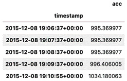
Figure 5.3 – The first five rows with a lowercase column name and an index

6. Note that the DataFrame has a timestamp as an index of the DatetimeIndex type. First, you will need to convert the index to a DataFrame column since the API does not support writing an index object, and because you do not want to lose that information, you will need to make it a column. Secondly, note that the column names are lowercase, which will generate an error when writing to Snowflake. You will need to at least have one uppercase letter in the name. To make it easier, just uppercase the column names:

   df = df.reset_index()

   df.columns = df.columns.str.upper()

   df.head()

The output is as follows:

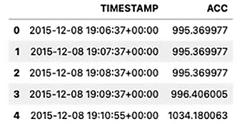
Figure 5.4 – The first five rows of the updated DataFrame with two uppercase columns

7. Write the DataFrame to Snowflake using the .to_sql() writer function. You will need to pass an insertion method; in this case, you will pass the pd_writer object:

   df.to_sql('sensor', 

               engine,

               index=False,

               method=pd_writer, 

               if_exists='replace')
8. To read and verify that the data was written, you can use pandas.read_sql() to query the table:

   query = 'SELECT * FROM SENSOR;'

   snow_df = pd.read_sql(query, engine, index_col='timestamp')

   snow_df.info()

   >> 

   <class 'pandas.core.frame.DataFrame'>

   DatetimeIndex: 3960 entries, 2015-12-08 19:06:37 to 2015-12-11 18:48:27

   Data columns (total 1 columns):

    #   Column  Non-Null Count  Dtype  

   ---  ------  --------------  -----  

    0   acc     3960 non-null   float64

   dtypes: float64(1)

   memory usage: 61.9 KB

Note that the timestamp is returned as a DatetimeIndex type.

How it works...

The Snowflake Python API provides two mechanisms for writing pandas DataFrames to Snowflake, which are provided to you from pandas_tools:

from snowflake.connector.pandas_tools import pd_writer, write_pandas

In the recipe, you used pd_writer and passed it as an insertion method to the DataFrame.to_sql() writer function. When using pd_writer within to_sql(), you can change the insertion behavior through the if_exists parameter, which takes three arguments:

• fail, which raises ValueError if the table exists
• replace, which drops the table before inserting new values
• append, which inserts the data into the existing table

If the table doesn't exist, SQLAlchemy takes care of creating the table for you and maps the data types from pandas DataFrames to the appropriate data types in the Snowflake database. This is also true when reading the data from Snowflake using the SQLAlchemy engine through pandas.read_sql().

Note that pd_writer uses the write_pandas function behind the scenes. They both work by dumping the DataFrame into Parquet files, uploading them to a temporary stage, and, finally, copying the data into the table via COPY INTO.

In the Reading data from Snowflake recipe in Chapter 3, Reading Time Series Data from Databases, we discussed how Snowflake, by default, stores unquoted object names in uppercase when these objects were created. Due to this, when using SQLAlchemy to write the DataFrame, you will need to either make the column names all uppercase or at least uppercase one character; otherwise, it will throw an error on the insert.

For example, if you did not uppercase the column names and used to_sql() to write to Snowflake, assuming the table did not exist, the table will be created along with the columns, all with uppercase letters, as shown in the following screenshot:

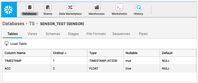
Figure 5.5 – Snowflake showing the uppercase column names

But when it comes to inserting the record, you will get a match error, as follows:

ProgrammingError: SQL compilation error: error line 1 at position 86
invalid identifier '"timestamp"'

From the preceding error, the culprit is the quoted column name, which does not match what is in Snowflake since, by default, Snowflake has them all uppercase. Here is an experiment you can do in Snowflake (Snowflake worksheets) to see the issue firsthand:

insert into sensor_test ("timestamp", "acc") values ('2015-12-08 19:06:37.000', '995.369977')
>> SQL compilation error: error line 1 at position 25 invalid identifier '"timestamp"'
insert into sensor_test ("TIMESTAMP", "ACC") values ('2015-12-08 19:06:37.000', '995.369977')

The first query will return the same error we received when using .to_sql(), while the second query is successfully executed. Figure 5.5 shows Snowflake's classic web interface. If you create a new Snowflake account, you will probably use the new Snowsight web interface by default. Of course, you can always switch to the classic console as well.

There's more...

The write_pandas function can be used to write (insert) data into a table similar to pd_writer, but in addition, it does return a tuple of (success, num_chunks, num_rows, output).

Using write_pandas does not leverage SQLAlchemy, so it assumes a table already exists to write the data into. Here is an example using write_pandas to write to the same sensor table:

from snowflake import connector
from snowflake.connector.pandas_tools import pd_writer, write_pandas
con = connector.connect(**params)
cursor = con.cursor()
# delete records from the previous write
cursor.execute('DELETE FROM sensor;')
success, nchunks, nrows, copy_into = write_pandas(con, df, table_name='SENSOR')

Print the returned values after the query has executed:

print('success: ', success)
print('number of chunks: ', nchunks)
print('number of rows: ', nrows)
print('COPY INTO output', copy_into)
>>
success:  True
number of chunks:  1
number of rows:  3960
COPY INTO output [('raeqh/file0.txt', 'LOADED', 3960, 3960, 1, 0, None, None, None, None)]

The information presented confirms the number of records written and the number of chunks, as well as output from the COPY INTO sensor statement.

In this recipe, you learned about two options for writing pandas DataFrames directly to Snowflake. The first was using the DataFrame.to_sql() writer function using SQLAlchemy, and the second was using Snowflake's connector and pd_writer() function.

See also

• For more information on write_pandas and pd_write, please visit the Snowflake documentation here: https://docs.snowflake.com/en/user-guide/python-connector-api.html#write_pandas.
• For more information on the pandas DataFrame.to_sql() function, please visit the pandas documentation here: https://pandas.pydata.org/docs/reference/api/pandas.DataFrame.to_sql.html.