Chapter 6: Third-Party Utilities

In the previous two chapters, we used tools and data provided by Microsoft to get insights into report performance. In this chapter, we will cover some popular freely available third-party utilities that complement the built-in offerings and improve your productivity when investigating report performance issues.

These tools have a range of features, such as documenting our solutions, analyzing them to give recommendations, the ability to modify Power BI artifacts, capturing performance traces, and running queries. It is beyond the scope of this book to cover the full functionality of these tools, so we will limit our coverage to features and techniques that help us assess and improve performance.

The utilities introduced in this chapter are largely maintained by community contributors and are often open source. All the utilities described in this chapter are widely used to the point where they are formally acknowledged by Microsoft. Power BI Desktop will recognize them if they are installed on your computer and allow you to launch them from its External Tools menu, sometimes even connected to the .pbix file you are working on. At the time of writing, these utilities are actively maintained, and the releases are generally of high quality.

However, while the development of these open source tools is often stewarded by experts who run their own Power BI consulting and training businesses, they are not always officially supported, so you should bear this in mind. Your organization may have policies against the use of such tools. If you do use them, be aware that you may not be able to get prompt dedicated assistance as you normally would with a support case for a paid commercial offering.

All the utilities in this chapter can connect to Analysis Services datasets running within Power BI Desktop, Azure Analysis Services, or the Power BI service. Therefore, we will simply refer to these tools connecting to Analysis Services datasets for most of the chapter.

This chapter is broken into the following sections:

• Power BI Helper
• Tabular Editor
• DAX Studio and VertiPaq Analyzer

Technical requirements

There are samples available for some parts of this chapter. We will call out which files to refer to. Please check out the Chapter06 folder on GitHub to get these assets: https://github.com/PacktPublishing/Microsoft-Power-BI-Performance-Best-Practices.

Power BI Helper

Power BI Helper has a range of features that help you explore, document, and compare local Power BI Desktop files. It also lets you explore and export metadata from the Power BI service, such as lists of workspaces and datasets and their properties. Power BI Helper can be downloaded from the following link: https://powerbihelper.org.

In previous chapters, we discussed how important it is to keep Power BI datasets smaller by removing unused tables and columns. Power BI Helper includes features to help you do this, so it could be a useful tool to incorporate into standard optimization processes before production releases.

Identifying large columns in the dataset

In general, having a smaller model speeds up report loads and data refresh, which is why it is good to be able to identify the largest items easily. For now, we simply want to introduce this capability so you are aware of this technique. We will learn about dataset size reduction in detail in Chapter 10, Data Modeling and Row-Level Security. Complete the following steps to investigate dataset size:

1. Open your .pbix file in Power BI Desktop, then connect Power BI Helper to the dataset.
2. Navigate to the Modeling Advise tab.
3. Observe how Power BI Helper lists all columns sorted by their dictionary size from largest to smallest.

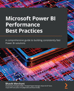
The dictionary size is how much space in MB is taken by the compressed data for that column. The following figure shows the result of this tab:

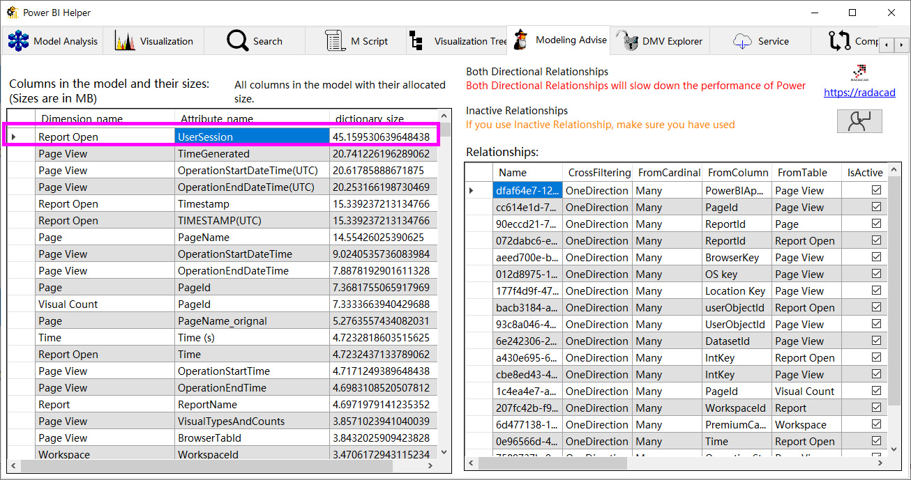
Figure 6.1 – Modeling Advise tab of showing largest column

In this example, the UserSession column (referred to as an attribute) takes up about 45 MB. The .pbix file was 172 MB. From these sizes, we can calculate that this one column contributes to approximately 25% of the file size, which is significant. You should try to remove large columns like this from the dataset. If you need it for reporting, relationship, or calculation purposes, try optimizing it using techniques from Chapter 10, Data Modeling and Row-Level Security.

Tip

A Power BI Desktop file in Import mode contains a complete copy of the source data. The data is contained within the .pbix file as an Analysis Services backup file (.abf). Even though the .pbix file size is not the same as the size of the dataset when it is loaded into memory, it can be used for a quick approximation to judge the impact of column and table sizes on the overall dataset size.

Identifying unused columns

Power BI Helper can identify all the unused columns in your model. You simply navigate to the Visualization tab and observe them in a list. You can remove them from the dataset by right-clicking the items and selecting Delete. This is shown in the following figure:

Figure 6.2 – Unused columns showing the ability to delete from Power BI Helper

Note that any changes applied in Power BI Helper will be applied to the .pbix file you have open immediately. By default, Power BI Helper will back up your original file to the location specified at the top left, as shown in the previous figure. It is recommended to use this backup feature to recover from accidental deletions.

Identifying bi-directional and inactive relationships

The Modeling Advise tab we referred to in Figure 6.1 has a relationships section on the right-hand side. You can use this to conveniently identify all bi-directional relationships in your dataset. These can slow down queries and might have unintentional filter consequences, so it's a good idea to review each one to ensure it is really needed.

Identifying measure dependencies

Power BI Helper visualizes measure dependencies via the Model Analysis tab. Measures can be reused within other measures, and this is the best practice for maintainability. In a chain of measure dependencies, the start of the chain is often referred to as the base measure. Base measures may be used in many other measures and Power BI Helper lets you easily identify all those reverse dependencies. You can use this information to get a better return on investment when performance tuning because optimizing base measures that are used in many other measures could have a large overall impact. Conversely, you may have a complex measure that uses many other measures. In this case, Power BI Helper helps you identify all the measures it uses so you know which to consider when optimizing.

We have seen how Power BI Helper can help us identify a few common dataset design issues. Next, we will look at Tabular Editor, another freely available tool that can go in more depth into dataset design guidance.

Tabular Editor

Tabular Editor is available as both a commercial offering and an open source version. The paid version offers some advanced development functionality and even dedicated support, which professional Power BI developers may find useful. The good news is that the free version contains all the useful core features at the time of writing, and it can be downloaded at the following GitHub link: https://github.com/TabularEditor/TabularEditor.

Tabular Editor is a productivity tool aimed at improving many aspects of the development experience offered by Power BI Desktop or Microsoft Visual Studio. These core features are out of scope for this book. Due to the sheer popularity of the tool with experienced BI developers, you are encouraged to learn more about Tabular Editor if you expect to build and maintain complex enterprise models over many months or even years. Please follow the product documentation to become familiar with the interface and functionality of Tabular Editor. We are going to focus on a specific feature of Tabular Editor called the Best Practice Analyzer.

Using Tabular Editor's Best Practice Analyzer

Tabular Editor has a powerful extension called the Best Practice Analyzer (BPA). This extension lets you define a set of modeling rules that can be saved as collections. An example of a rule is to avoid using floating-point data types for numerical columns. Once you have a set of rules defined, you can use the BPA to scan an Analysis Services dataset. It will check all objects against applicable modeling rules and generate a report in the process.

After you have installed Tabular Editor, open the Tools menu. Here you will find the options to launch the BPA and manage its rules, as shown in the following figure:

Figure 6.3 – How to manage BPA rules in Tabular Editor

If this is the first time you are using Tabular Editor, you will find that there are no rules included with the installer. The best way to start is to use a default set of best practices that Microsoft helped define, and you need to perform some brief manual steps to load in some default rules. For reference, you can find the rules included within the Tabular Editor project on GitHub, at the following location: https://github.com/TabularEditor/BestPracticeRules.

To install the rules, you simply copy the BPARules.json file found at the previous link into the %localappdata%TabularEditor folder on your computer. You can paste this exact location into Windows File Explorer to get to the appropriate place.

Alternatively, you can use the Advanced Scripting functionality of Tabular Editor to download and copy the rules to the location for you. Simply paste the following script into the tool, run it, then restart Tabular Editor to have the rules available:

System.Net.WebClient w = new System.Net.WebClient();

string path = System.Environment.GetFolderPath(System.Environment.SpecialFolder.LocalApplicationData);

string url = "https://raw.githubusercontent.com/microsoft/Analysis-Services/master/BestPracticeRules/BPARules.json";

string downloadLoc = path+@"TabularEditorBPARules.json";

w.DownloadFile(url, downloadLoc);

Note

You need to connect to an Analysis Services dataset in Tabular Editor before you can run any scripts; otherwise, the option will be disabled in the toolbar.

The following figure shows the result of running the BPA download script in Tabular Editor, highlighting the script execution button and the successful result shown in the status bar:

Figure 6.4 – BPA rules successfully loaded via the Advanced Scripting feature

Once you have the rules loaded, you can view, modify, and add rules as you please. The following screenshots show what the interface looks like after rules are imported:

Figure 6.5 – BPA rules loaded into Tabular Editor

The next screenshot shows the rule editor, after opening an existing rule:

Figure 6.6 – Editing a best practice rule

When you want to run the BPA rules against your dataset, connect to it using one of the supported methods in Tabular Editor. Once connected, run the BPA by pressing F10 or by selecting it from the Tools menu, which was introduced in Figure 6.3.

A sample of results that can be obtained from running the BPA on a dataset is shown in the following figure. It highlights three useful toolbar buttons that are available for some rules:

• Go to object: This will open the model script at the definition of the offending object.
• Generate fix script: This will generate a script you can use to apply the change and copy it to the clipboard.
• Apply fix: This will apply the fix script to your model immediately. Be careful with this option and make sure you have a backup in place beforehand.

Figure 6.7 – BPA results, highlighting context-sensitive toolbar actions

Once you have the BPA results, you need to decide which changes to apply. It might seem like a great idea to simply apply all changes automatically. However, we advise a careful review of the results and applying some thought to which recommendations to apply and in what order.

The default BPA rules are grouped into six categories:

• DAX Expressions
• Error Prevention
• Formatting, Maintenance
• Naming Conventions
• Performance

For performance optimization, we advise focusing on the Performance and DAX Expressions categories. These optimizations have a direct impact on the query and refresh performance. The other categories benefit usability and maintenance.

Tip

The best way to be certain that performance optimizations have had the expected impact is to test the effect of each change in typical usage scenarios. For example, if you plan to optimize three independent DAX measures, change one at a time and check the improvement you get with each change. Then check again with all changes applied. This will help you identify the most impactful change and not assume that every change will result in a measurable difference when stacked with others. This will also help you learn the relative impact of design patterns, so you know what to look for first next time around to get the best return on investment when optimizing designs.

Thus far, we have been introduced to some utilities that help us identify dataset design issues. Next, we will look at DAX Studio and VertiPaq Analyzer. These are complementary tools that give us more dataset information and help us debug and resolve dataset and DAX performance issues, with the ability to customize DAX queries and measure their speed.

DAX Studio and VertiPaq Analyzer

DAX Studio, as the name implies, is a tool centered around DAX queries. It provides a simple yet intuitive interface with powerful features to browse and query Analysis Services datasets. We will cover querying later in this section. For now, let's look deeper into datasets.

The Analysis Services engine has supported Dynamic Management Views (DMVs) for many years. These views refer to SQL-like queries that can be executed on Analysis Services to return information about dataset objects and operations.

VertiPaq Analyzer is a utility that uses publicly documented DMVs to display essential information about which structures exist inside the dataset and how much space they occupy. It started life as a standalone utility, published as a Power Pivot for an Excel workbook, and still exists in that form today. In this chapter, we will refer to its more recent incarnation as a built-in feature of DAX Studio.

It is interesting to note that VertiPaq is the original name given to the compressed column storage engine within Analysis Services (Verti referring to columns and Paq referring to compression).

Analyzing model size with VertiPaq Analyzer

VertiPaq Analyzer is now built into DAX Studio as the View Metrics feature, found in the Advanced tab of the toolbar. You simply click the icon to have DAX Studio run the DMVs for you and display the statistics in a tabular form. This is shown in the following figure:

Figure 6.8 – Using View Metrics to generate VertiPaq Analyzer stats

You can switch to the Summary tab of the Vertipaq Analyzer Metrics pane to get an idea of the overall total size of the model along with other summary statistics, as shown in the following figure:

Figure 6.9 – Summary tab of VertiPaq Analyzer Metrics

The Total Size metric provided in the previous figure will often be larger than the size of the dataset on disk (as a .pbix file or Analysis Services .abf backup). This is because there are additional structures required when the dataset is loaded into memory, which is particularly true of Import mode datasets.

In Chapter 2, Exploring Power BI Architecture and Configuration, we learned about Power BI's compressed column storage engine. The DMV statistics provided by VertiPaq Analyzer let us see just how compressible columns are and how much space they are taking up. It also allows us to observe other objects, such as relationships.

The Columns tab is a great way to see whether you have any columns that are very large relative to others or the entire dataset. The following figure shows the columns view for the same dataset we saw in Figure 6.9. You can see how from 238 columns, a single column called Operation-EventText takes up a staggering 39% of the whole dataset size! It's interesting to see its Cardinality (or uniqueness) value is about four times lower than the next largest column's:

Figure 6.10 – One column monopolizing the dataset

In the previous figure, we can also see that Data Type is String, which is alphanumeric text. These statistics would lead you to deduce that this column contains long, unique text values that do not compress well. Indeed, in this case, the column contained DAX and DQ query text from Analysis Services engine traces that were loaded into Power BI. A finding such as this may lead you to re-evaluate the need for this level of detail in the dataset. You'd need to ask yourself whether the extra storage space and time taken to build the compressed columns and potentially other structures is worth it for your business case. In cases of highly detailed data such as this where you do need long text values, consider limiting the analysis to shorter time periods, such as days or weeks.

Now let's learn about how DAX Studio can help us with performance analysis and improvement.

Performance tuning the data model and DAX

The first-party option for capturing Analysis Services traces is SQL Server Profiler. When starting a trace, you must identify exactly which events to capture, which requires some knowledge of the trace events and what they contain. Even with this knowledge, working with the trace data in Profiler can be tough since the tool was designed primarily to work with SQL Server database traces. The good news is that DAX Studio can start an Analysis Services server trace then parse and format all the data to show you relevant results well presented within its user interface. It allows us to both run and measure queries in a single place and provides bespoke features for Analysis Services that make it a good alternative SQL Profiler for tuning Analysis Services datasets.

Capturing and replaying queries

The All Queries command in the Traces section of the DAX Studio toolbar will start a trace against the dataset you have connected to. The following figure shows the result when a trace is successfully started:

Figure 6.11 – Query trace successfully started

Once your trace has started, you can interact with the dataset outside DAX Studio and it will capture queries for you. How you interact with the dataset depends on where it is. For a dataset running on your computer in Power BI Desktop, you would simply interact with the report. This would generate queries that DAX Studio will see. The All Queries tab at the bottom of the tool is where the captured queries are listed in time order with durations in milliseconds. The following figure shows two queries captured when opening the Unique by Account No page from the Slow vs Fast Measures.pbix sample file:

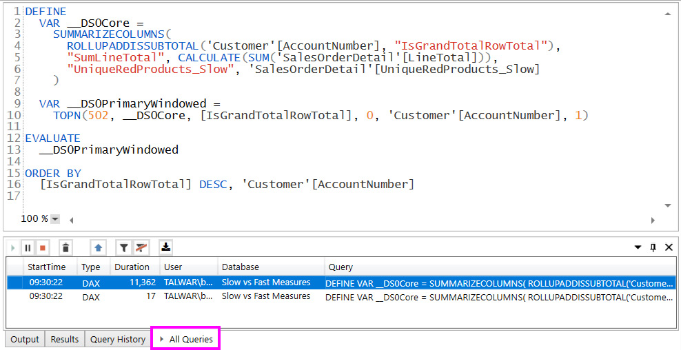
Figure 6.12 – Queries captured by DAX Studio

In Chapter 5, Desktop Performance Analyzer, we presented Figure 5.9 in the section entitled Interpreting and acting on performance analyzer data. It showed two visuals that generated the same output onscreen. The previous screenshot shows us that the fast version took only 17 ms whereas the slow version tool took more than 11.3 seconds. In the screenshot, the query selected in blue was double-clicked to bring its DAX text into the editor above. You can now modify this query in DAX Studio to test performance changes. We learned in the previous chapter that the DAX expression for the UniqueRedProducts_Slow measure was not efficient. We'll learn a technique to optimize queries soon, but first, we need to learn about capturing query performance traces.

Obtaining query timings

To get detailed query performance information, you can use the Server Timings command shown in Figure 6.12. After starting the trace, you can run queries and then use the Server Timings tab to see how the engine executed the query, as shown in the following figure:

Figure 6.13 – Server Timings showing detailed query performance statistics

The previous figure gives very useful information. FE and SE refer to the formula engine and storage engine. The storage engine is fast and multi-threaded, and its job is fetching data. It can apply basic logic such as filtering data to retrieve only what is needed. The storage engine is single-threaded and it generates a query plan, which is the physical steps required to compute the result. It also performs calculations on the data such as joins, complex filters, aggregations, and lookups. We want to avoid queries that are spending most of the time in the formula engine, or that execute many queries in the storage engine. The bottom-left section of Figure 6.14 shows that we executed almost 5,000 SE queries. The list of queries to the right shows many queries returning only one result, which is suspicious.

For comparison, we look at timings for the fast version of the query and we see the following:

Figure 6.14 – Server Timings for fast version of query

In the previous screenshot, we can see that only three server engine queries were run this time, and the result was obtained much faster.

Tip

The Analysis Services engine does use data caches to speed up queries. These caches contain uncompressed query results that can be reused later to save time fetching and decompressing data. You should use the Clear Cache button in DAX Studio to force these caches to be cleared and get a proper worst-case performance measure. This is visible in the menu bar in Figure 6.12.

We will build on these concepts when we look at DAX and model optimizations in later chapters. Now let's look at how we can experiment with DAX and query changes in DAX Studio.

Modifying and tuning queries

Earlier in the section, we saw how we could capture a query generated by a Power BI visual then display its text. A nice trick we can use here is to use query-scoped measures to override the measure definition and see how performance differs.

The following screenshot shows how we can search for a measure, right-click, then pull its definition into the query editor:

Figure 6.15 – Define Measure option and result in Query pane

We can now modify the measure in the query editor, and the engine will use the local definition instead of the one defined in the model! This technique gives you a fast way to prototype DAX enhancements without having to edit them in Power BI and refresh visuals over many iterations.

Do remember that this technique does not apply any changes to the dataset you are connected to. You can optimize expressions in DAX Studio, then transfer the definition to Power BI Desktop/Visual Studio when ready. The following screenshot shows how we changed the definition of UniqueRedProduct_Slow in a query-scoped measure to get a huge performance boost:

Figure 6.16 – Modified measure giving better results

The techniques described here can be adapted to model changes too. For example, if you wanted to determine the impact of changing a relationship type, you could run the same queries in DAX Studio before and after the change to draw a comparison.

Here are some additional tips for working with DAX Studio:

• Isolate measures: When performance tuning a query generated by a report visual, comment out complex measures and then establish a baseline performance score. Then add each measure back to the query individually and check the speed. This will help identify the slowest measures in that query and visual context.
• Work with Desktop Performance Analyzer traces: DAX Studio has a facility to import the trace files generated by Desktop Performance Analyzer. You can import the trace files using the Load Perf Data button located next to All Queries highlighted in Figure 6.11. This trace can be captured by one person then shared with a DAX/modeling expert who can use DAX Studio to analyze and replay their behavior. The following figure shows how DAX Studio formats the data to make it easy to see which visual and component is taking the most time. It was generated by viewing each of the three report pages in the Slow vs Fast Measures.pbix sample file:

Figure 6.17 – Performance Analyzer trace shows slowest visual caused by slow query

• Export/import model metrics: DAX Studio has a facility to export or import the VertiPaq model metadata using .vpax files. These files do not contain any of your data. They contain table names, column names, and measure definitions. If you are not concerned with sharing these definitions, you can provide .vpax files to others if you need assistance with model optimization.

We have now seen how we can use useful free tools to learn more about our Power BI solutions and identify areas to improve. Let's summarize and review our learnings from the chapter.

Summary

In this chapter, we introduced some popular utilities that use different methods to analyze Power BI solutions and help us identify areas to improve. They are complementary to those provided by Microsoft and can enhance our optimization experience.

We learned that these tools are mature and have a broad range of functionality beyond performance improvement, so you are encouraged to explore all their features and consider incorporating them into your development cycle. One caveat is that free versions of these tools are often community projects and are not officially supported.

We learned about Power BI Helper and its ability to identify large columns, unused columns, bi-directional relationships, and measure dependencies. These are all candidates for performance improvement.

Next, we learned about Tabular Editor and its built-in BPA. This gave us an easy way to load in default rules provided by experts, then scan a dataset for a range of performance and other best practices. BPA could even apply some fixes immediately if desired.

Then we were introduced to DAX Studio and VertiPaq Analyzer. DAX Studio is a complete query development and tuning utility that can capture real-time query activity from Power BI datasets, including server timings. We learned how to generate dataset metrics that give us detailed information about the objects in the dataset and how much space they occupy. We then moved on to query timings, so we learned about the roles of the formula engine and the storage engine and how to see how much time is spent in each. We could also see the internal VertiPaq queries that were executed. The ability to use query-scoped measures in DAX Studio gives us a fast and powerful way to prototype DAX and model changes and see their impact on the engine timings.

At this point in the book, we learned about optimizing Power BI largely from a high-level design perspective. We also learned about tools and utilities to help us measure performance. In the next chapter, we will propose a framework where you will combine processes and practices that use these tools to establish, monitor, and maintain good performance in Power BI.