
Chapter 11: Improving DAX
In the previous chapter, we focused on Import datasets at the visual layer in Power BI, where a key point was to reduce the load on data sources by minimizing the complexity and number of queries that are issued to the Power BI dataset.
In theory, a well-designed data model should not experience performance issues easily unless there are extremely high data volumes with tens of millions of rows or more. However, it is still possible to get poor performance with good data models due to the way DAX measures are constructed.
Learning DAX basics is considered quite easy by many people. It can be approached by people without a technical data background but who are comfortable writing formulas in a tool such as Microsoft Excel. However, mastering DAX can be challenging. This is because DAX is a rich language with multiple ways to achieve the same result. Mastery requires having knowledge of row context and filter context, which determines what data is in scope at a point in the execution. In Chapter 6, Third-Party Utilities, we talked about the formula engine and storage engine in Analysis Services. In this chapter, we will look at examples of how DAX design patterns and being in filter context versus row context can affect how the engine behaves. We will see where time is spent in slower versus faster versions of the same calculation.
We will also identify DAX patterns that typically cause performance problems and how to rewrite them.
This chapter contains a single section presented as a collection of performance tips:
- Understanding DAX pitfalls and optimizations
Technical requirements
There is one combined sample file available for this chapter and all the sample references can be found in the DAX Optimization.pbix file, in the Chapter11 folder in this book's GitHub repository: https://github.com/PacktPublishing/Microsoft-Power-BI-Performance-Best-Practices.
Understanding DAX pitfalls and optimizations
Before we dive into specific DAX improvements, we will briefly review the following suggested process to tune your DAX formulas.
The process for tuning DAX
In Chapter 5, Desktop Performance Analyzer, and Chapter 6, Third-Party Utilities, we provided detailed information and examples of how to use various tools to measure performance. We'll take this opportunity to remind you of which tools can help with DAX tuning and how they can be used. A recommended method to tune DAX is as follows:
- Review the DAX expressions in the dataset. Ideally, run the Best Practice Analyzer (BPA) to identify potential DAX improvements. The BPA does cover some of the guidance provided in the next section, but it's a good idea to check all the rules manually.
- Rank the suggestions in terms of estimated effort, from lowest to highest. Consider moving some calculations or even intermediate results to Power Query. This is usually a better place to perform row-by-row calculations.
- In a development version of the data model, implement trivial fixes right away, but always check your measures to make sure they are still providing the same results.
- Using the Power BI Desktop Performance Analyzer, check the performance of the report pages and visuals. Copy the queries that have been captured by the Analyzer into DAX Studio. Then use the Server Timings feature in DAX Studio to analyze load on the formula engine versus storage engine.
- Modify your DAX expressions and confirm that performance has improved in DAX Studio – remember that DAX Studio allows you to safely overwrite measures locally without changing the actual dataset.
- Make DAX changes in the dataset and check the report again with Performance Analyzer to ensure there are no unexpected performance degradations and that the results are still correct.
- Test the changes in a production-like environment using realistic user scenarios and data volumes. If successful, deploy to the updates; otherwise, repeat the process to iron out any remaining issues.
Now, let's review DAX guidance.
DAX guidance
We will continue with the theme of having the Analysis Services engine do as little work as possible, with as little data as possible. Even with optimized datasets that follow good data modeling practices, inefficient DAX can make the engine unnecessarily scan rows, or perform slow logic in the formula engine. Therefore, our goals for tuning DAX are as follows:
- Reduce the work that's done by the single-threaded formula engine.
- Reduce the total number of internal queries that are generated by a DAX query.
- Avoid scanning large tables.
Note
In this section, we will only show the DAX Studio performance results for the first few tips. Please be aware that you can use DAX Studio, Desktop Performance Analyzer, and other tools to measure performance and tune DAX for all the cases mentioned here.
The following list represents some common design choices that lead to lower performance. We will explain why each one can be problematic and what you can do instead:
- Use variables instead of repeating measure definitions: Sometimes, when we are performing a calculation, we need to reuse a calculated value multiple times to get to the result. We will use an example where we have some sales figures and need to calculate the variance percentage compared to the same period in the previous year. One way to write this calculation is as follows:
YoY% =
(
SUM('Fact Sale'[Total Sales])
- CALCULATE(SUM('Fact Sale'[Total Sales]), DATEADD('Dimension Date'[Date], -1, YEAR))
),
/
CALCULATE(SUM('Fact Sale'[Total Sales]), DATEADD('Dimension Date'[Date], -1, YEAR)
Observe that we are referencing the prior year's sales value twice – once to calculate the numerator and again to calculate the denominator. This makes the engine duplicate some effort and might not take full advantage of caching in Analysis Services. A better way of doing this would be to use a variable. Note that we have not handled error cases and fully optimized this yet:
YoY% VAR =
VAR __PREV_YEAR =
CALCULATE(
SUM('Fact Sale'[Total Sales]),
DATEADD('Dimension Date'[Date], -1, YEAR))
RETURN
(SUM('Fact Sale'[Total Sales]) - __PREV_YEAR) /__PREV_YEAR
The difference here is that we have introduced the VAR statement to define a variable called __PREV_YEAR, which will hold the value of last year's sales. This value can be reused anywhere in the formula simply by name, without incurring recalculation.
You can see this in action in the sample file, which contains both versions of the measure. The Without Variable and With Variable report pages contain a table visual, like this:

Figure 11.1 – Table visual showing a year-on-year % growth measure
We captured the query trace information in DAX Studio to see how these perform. The results can be seen in the following screenshot:

Figure 11.2 – DAX Studio showing less work and duration with a variable
In the preceding screenshot, the first query without the variable was a bit slower. We can see it executed one extra storage engine query, which does appear to have hit a cache in our simple example. We can also see more time being spent in the formula engine than with the version with a variable. In our example, where the fact table contains about 220,000 rows, this difference would be unnoticeable. This can become significant with higher volumes and more sophisticated calculations, especially if a base measure is used in other measures that are all displayed at the same time.
Note
Using variables is probably the single most important tip for DAX performance. There are so many examples of calculations that need to use calculated values multiple times to achieve the desired result. You will also find that Power BI automatically uses this and other recommended practices in areas where it generates code for you, such as Quick Measures.
- Use DIVIDE instead of the division operator: When we divide numbers, we sometimes need to avoid errors by checking for blank or zero values in the denominator. This results in conditional logic statements, which add extra work for the formula engine. Let's continue with the example from Figure 11.1. Instead of year-on-year growth, we now want to calculate a profit margin. We want to avoid report errors by handling blank and zero values:
Profit IF =
IF(
OR(
ISBLANK([Sales]),[Sales] == 0
),
BLANK(),
[Profit]/[Sales]
)
An improved version would use the DIVIDE function, as follows:
Profit DIVIDE =
DIVIDE([Profit], [Sales])
This function has several advantages. It automatically handles zero and blank values at the storage engine layer, which is parallel and faster. It has an optional third parameter that allows you to specify an alternative value to use if the denominator is zero or blank. It is also a much shorter measure that is easier to understand and maintain.
When we take a look at the performance numbers from DAX Studio, we can see stark differences. The first version is nearly three times slower than the optimized version, as shown in the following screenshot:

Figure 11.3 – DAX Studio showing less work done by DIVIDE
The preceding screenshot also shows us that the slower version issued more internal queries and spent about four times longer in the storage engine. It also spent about twice as much time in the formula engine. Once again, this is just a single query for one visual. This difference can be compounded for a typical report page that runs many queries. You can experiment with this using the Profit IF and Profit DIVIDE pages in the sample file.
- For numerical measures, avoid converting blank results into zero or some text value: Sometimes, for usability reasons, people write measures with conditional statements to check for a blank result and replace it with zero. This is more common in financial reporting, where people need to see every dimensional value (for example, Cost Code or SKU), regardless of whether any activity occurred. Let's look at an example. We have a simple measure called Sales in our sample file that sums the 'Fact Sale'[Total Including Tax] column. We have adjusted it to return zero instead of blanks, as follows:
SalesNoBlank =
VAR SumSales =
SUM('Fact Sale'[Total Including Tax])
RETURN
IF(ISBLANK(SumSales), 0, SumSales)
Then, we constructed a matrix visual that shows sales by product barcode for both versions of the measure. The results are shown in the following screenshot. At the top, we can see the values for 2016, which implies there are no sales for these product bar codes in other years. At the bottom, we can see 2013 onwards, which we can scroll through:

Figure 11.4 – The same totals but many more rows when replacing blanks
Both results shown in the preceding screenshot are technically correct. However, there is a performance penalty for replacing blanks. If we think about a dimensional model, in theory, we could record a fact for every possible combination of dimensions. In practical terms, for our Sales example, in theory, we could sell things every single day, for every product, for every employee, in every location, and so on. However, there will nearly always be some combinations that are not realistic or simply don't have activities against them. Analysis Services is highly optimized to take advantage of empty dimensional intersections and doesn't return rows for combinations where all the measures are blank. We measured the query that was produced by the visuals in the preceding screenshot. You can see the performance difference in DAX Studio in the following screenshot:

Figure 11.5 – Slower performance when replacing blanks
The preceding screenshot shows a longer total duration, more queries executed, and significantly more time spent in the formula engine. You can see these on the MeasureWithBlank and MeasureNoBlank report pages in the sample file.
Consider not replacing blanks in your measure but solving this problem on a per-visual basis. You can do this by selecting a visual and using the Fields pane in Power BI Desktop to enable Show items with no data for specific attributes of a dimension, as shown in the following screenshot. This change will still produce a less optimal query, but not one that's quite as slow as using measures:
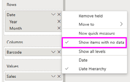
Figure 11.6 – Show items with no data
Another advantage of the visual-based approach is that you are not forced to take a performance hit everywhere the measure is used. You can balance performance with usability selectively.
If you still need to implement blank handling centrally, you could consider making the measures more complex to only substitute a blank for the correct scope of data. We recommended checking out the detailed article from SQLBI on this topic, which shows a combination of DAX and data modeling techniques to use, depending on your scenario: https://www.sqlbi.com/articles/how-to-return-0-instead-of-blank-in-dax.
A final point here is to avoid replacing blanks in numerical data with text values such as No data. While this can be helpful for users, it can be even slower than substituting zero because we are forcing the measure to become a string. This can also create problems downstream if the measure is used in other calculations.
- Use SELECTEDVALUE instead of VALUES: Sometimes, a calculation is only relevant when a single item from a dimension is in scope. For example, you may use a slicer as a parameter table to allow users to dynamically change measures, such as scaling by some factor. One pattern to access the single value in scope is to use HASONEVALUE to check for only one value, and then use the VALUES DAX function. If we had a parameter table called Scale, our measure would look like this:
Sales by Scale =
DIVIDE (
[Sales Amount],
IF( HASONEVALUE ( Scale[Scale] ), VALUES ( Scale[Scale] ), 1 )
)
Instead, we suggest that you use SELECTEDVALUE, which performs both steps internally. It returns blank if there are no items or multiple items in scope and allows you to specify an alternate value if there are zero or multiple items in scope. A better version is as follows:
Sales by Scale =
DIVIDE (
[Sales],
SELECTEDVALUE ( 'Scale'[Scale], 1 )
)
You can see this technique in use in the sample file on the SELECTEDVALUE report page.
- Use IFERROR and ISERROR appropriately: These are helpful functions that a data modeler can use to catch calculation errors. They can be wrapped around a measure to provide alternatives if there are calculation errors. However, they should be used with care because they increase the number of storage engine scans required and can force row-by-row operations in the engine. We recommend dealing with data errors at the source or in the ETL stages to avoid performing error checking in DAX. This may not always be feasible, so depending on the situation, you should try to use other techniques, such as the following:
- The FIND or SEARCH functions to search for and substitute values for failed matches
- The DIVIDE or SELECTEDVALUE functions to handle zeros and blanks
- Use SUMMARIZE only for text columns: This is the original function that's included in DAX to perform grouping. While it allows any column type, we advise not using numerical columns for performance reasons. Instead, use SUMMARIZECOLUMNS, which is newer and more optimized. There are many examples and use cases here, so we recommend checking out the following article by SQLBI, which provides much deeper coverage: https://www.sqlbi.com/articles/introducing-summarizecolumns.
- Avoid FILTER in functions that accept filter conditions: Functions such as CALCULATE and CALCULATETABLE accept a filter parameter that is used to adjust the context of the calculation. The FILTER function returns a table, which is not efficient when it's used as a filter condition in other functions. Instead, try to convert the FILTER statement into a Boolean expression. Consider the following measure:
Wingtip Sales FILTER =
CALCULATE(
[Sales],
FILTER('Dimension Customer', 'Dimension Customer'[Buying Group] == "Wingtip Toys")
)
It is better to replace the table expression with a Boolean expression, as follows:
Wingtip Sales =
CALCULATE(
[Sales],
'Dimension Customer'[Buying Group] == "Wingtip Toys")
)
The FILTER function can force row-by-row operations in the engine, whereas the improved Boolean version will use more efficient filtering on the column stores.
- Use COUNTROWS instead of COUNT: We often write measures to count the number of rows in a table within a context. Two choices will provide the same result, but only if there are no blank values. The COUNT function accepts a column reference, whereas the COUNTROWS function accepts a table reference. When you need to count rows and do not care about blanks, the latter will perform better.
- Use ISBLANK instead of = BLANK to check for empty values: They achieve the same result, but ISBLANK is faster.
- Optimize virtual relationships with TREATAS: There are times when we need to filter a table based on column values from another table but cannot create a physical relationship in the dataset. It may be that multiple columns are needed to form a unique key, or that the relationship is many-to-many. You can solve this using FILTER and CONTAINS, or INTERSECT. However, TREATAS will perform better and is recommended.
Look at the TREATAS report page in our sample file. The following screenshot shows an example where we added a new table to hold rewards groupings for customers based on their Buying Group and Postal Code. We want to filter sales using a new Reward Group column. We will not be able to build a single relationship with more than one key field:

Figure 11.7 – The new Reward Group table cannot be connected to the Customer table
We can write a measure to handle this using CONTAINS, as follows:
RG Sales CONTAINS =
CALCULATE(
[Sales],
FILTER(
ALL('Dimension Customer'[Buying Group]),
CONTAINS(
VALUES(RewardsGroup[Buying Group]),
RewardsGroup[Buying Group],
'Dimension Customer'[Buying Group]
)
),
FILTER(
ALL('Dimension Customer'[Postal Code]),
CONTAINS(
VALUES(RewardsGroup[Postal Code]),
RewardsGroup[Postal Code],
'Dimension Customer'[Postal Code]
)
)
)
This is quite long for a simple piece of logic, and it does not perform that well. A better version that uses TREATAS would look like this:
RG Sales TREATAS =
CALCULATE(
[Sales],
TREATAS(
SUMMARIZE(RewardsGroup, RewardsGroup[Buying Group], RewardsGroup[Postal Code]),
'Dimension Customer'[Buying Group],
'Dimension Customer'[Postal Code]
)
)
We haven't shown the INTERSECT version here, but note that it will be a little easier to write and can provide better performance. However, the TREATAS version is much shorter and easier to read and maintain. It will also perform better. Here, we visualized a simple table, as shown in the following screenshot, and managed to get nearly a 25% speed improvement with TREATAS. We also reduced the number of storage engine queries from 11 to 8:

Figure 11.8 – The visual that was used to test CONTAINS versus TREATAS performance
Now that we have learned about DAX optimizations, let's summarize what we've learned in this chapter.
Summary
In this chapter, we learned that DAX tuning is important because inefficient formulas can impact performance, even with well-designed datasets. This is because the DAX pattern directly influences how Analysis Services retrieves data and calculates query results.
We looked at a process for DAX tuning using tools that were introduced earlier in this book. First, we suggested using the Best Practice Analyzer and manual reviews to identify DAX improvements and then prioritize the changes to handle trivial fixes. Then, we suggested using Desktop Performance Analyzer to capture the queries that have been generated by visuals and running them in DAX Studio to understand their behavior. It is important to look at the total duration, number of internal queries, and time spent in the formula engine versus the storage engine. Once the changes have been prototyped and verified in DAX Studio, they can be made in the dataset; reports should be checked in production scenarios for performance gains.
Next, we looked at a range of common DAX pitfalls and alternative designs that can improve performance. We learned that, in general, we are trying to avoid formula engine work and wish to reduce the number of storage engine queries. Whenever possible, we explained why a performance penalty is incurred. We also provided examples of visual treatments and DAX Studio results for common optimizations to help you learn where to look, and what to look for.
Considering what we've learned so far, there may still be issues where the sheer volume of data can cause problems where additional modeling and architectural approaches need to be used to provide acceptable performance. Therefore, in the next chapter, we will look at techniques that can help us manage big data that reaches the terabyte scale.