Chapter 12: Exploring Storage and Database Options in GCP – Part 2

In the first part of our storage and database exploration, we looked at several services. In this chapter, we will focus on the remaining core database options.

The concepts of these services may sound similar to those we discussed in the previous chapter. For example, Cloud Spanner has similarities to Cloud SQL, while Bigtable may have you thinking about Cloud Datastore. In this chapter, we will not only look at the Cloud Spanner and Bigtable services but also show you how they differ and why you may need to select these over the other offerings.

We cover the following topics in this chapter:

• Cloud Spanner
• Bigtable

Cloud Spanner

There may be situations where you require horizontal scaling and Cloud SQL will not fit these requirements. Enter Cloud Spanner. Cloud Spanner is a cloud-native, fully managed offering that is designed specifically to combine relational database features, such as support for ACID transactions and SQL queries, with the horizontal scaling of a non-relational database. We should look to use Cloud Spanner when we have requirements for high queries per second or to deliver over multiple regions. Unlike most databases, Cloud Spanner is globally distributed and provides a strongly consistent database service with high performance.

Important Note

To reiterate, Cloud Spanner is strongly consistent.

It also offers an availability SLA of >=99.999% when you're using a multi-regional instance and is capable of providing up to 10,000 queries per second of reads or 2,000 queries per second of writes. It is important to understand that Cloud Spanner is SQL-like and has a schema; however, because of its high availability, it is ideal for mission-critical workloads. Its key use cases are from the financial and retail industries.

Exam Tip

With horizontal scalability, it will also support applications hosting across multiple regions. Remember that Cloud Spanner is ideal for workloads that require strong consistency.

Let's look at the configuration Cloud Spanner. We must create a Cloud Spanner instance inside our GCP project to do this.

Instance configurations

When we create a new instance, we should select an instance configuration. This will determine where our instance will reside and the replication of the databases in the instance. We can select between the following:

• Multi-regional: By using this instance, we will gain a higher SLA of 99.999% – or a downtime of approximately 5 minutes per year – but it will be more costly. Multi-regional allows the database's data to be replicated in multiple zones across multiple regions, allowing us to read data with low latency from locations. However, because replicas will be spread across more than one region, our applications will see a small increase in write latency.
• Regional: This will result in a 99.99% SLA, which is still very high and equivalent to approximately only 52 minutes of downtime per year. Regional instances should be selected if users and services are within the same region. This will offer the lowest latency. As you can see, the requirements will dictate the best option. We cannot change the instance's configuration after creation. Regional configurations will contain three read/write replicas that allow us to meet any governance requirements regarding where our data is located.

Node count

We are also required to select the number of nodes to allocate to our instance. This will determine the amount of CPU/RAM and storage resources that are available to our instance. Each node will provide up to 2 TB of storage, and it is recommended that a minimum of three nodes be used for production environments. We can change the number of nodes after creation to scale up or down.

Processing units

Cloud Spanner now supports processing units. 1,000 processing units is equivalent to 1 node and each increment of 100 units will behave like 1/10th of a node.

Replication

We mentioned replicas previously, and it's important to take a closer look at replication within Cloud Spanner. The underlying distributed filesystem that Cloud Spanner is built on will automatically replicate at the byte level. However, to provide additional data availability and geographic locality, Cloud Spanner will also replicate data by creating copies (replicas) of the rows that Cloud Spanner organized data into. These copies are then stored in a different geographic area. One of these replicas is elected to act as the leader and will be responsible for handling writes. Cloud Spanner has three types of replicas:

• Read/Write: This type of replication will maintain a full copy of our data and is eligible to become a leader. This is the only type of replication that's available to single-region instances.
• Read-Only: This type of replication will only support reads and cannot become a leader. It will maintain a full copy of our data, which has been replicated from our read/write replica. Read-Only is only available in multi-regional configurations.
• Witness: This type of replication doesn't support reads, nor does it maintain a full copy of our data. Witness replication makes it easier for us to achieve quorums for writes without the compute resources that are required by a read/write replica. Witness is only available in multi-regional configurations.

TrueTime

TrueTime is a globally distributed clock built on GPS and atomic clocks. It returns a time interval that is guaranteed to contain the clock's actual time. TrueTime is provided to applications on Google Servers, which allows applications to generate monotonically increasing timestamps. Cloud Spanner uses TrueTime to assign timestamps to transactions whenever Cloud Spanner deems the transaction to have taken place.

Data consistency

If you are looking for guaranteed strong consistency, then Cloud Spanner is the database offering for you! This is all down to the fact it is designed for the cloud and, therefore, will negate a lot of the constraints of other database offerings. Note that Cloud Spanner provides external consistency, which is a stronger property than strong consistency. This is the strictest consistency property for transaction-processing systems.

When we speak about data consistency concerning Cloud Spanner, it is wise to raise awareness of the concept of the CAP theorem. This theorem says that a database can only have two out of three of the following properties:

• C: Consistency. This implies a single value for shared data.
• A: Availability. 100% for both reads and updates.
• P: Partitions. Tolerance for network partitions.

This means that systems can be made up of CA, CP, or AP. The theorem is about 100% availability, but we know that systems will not offer 100% availability; therefore, system developers are forced to think seriously about the trade-off. If we believe that some network partitions are inevitable at some point in a system's life cycle, then a distributed system should be designed to forfeit consistency or availability – but only during a partition. Cloud Spanner, in times of a partition, will forfeit availability to ensure consistency. Given that Spanner offers 99.999% availability, which equates to less than 5.26 minutes of downtime per year, this is deemed to be high enough that we don't need to worry about availability trade-offs.

Encryption

By default, all data in Cloud Spanner will use Google-managed default encryption. When Customer-Managed Encryption Keys (CMEK) are enabled, Cloud Spanner will use our Cloud Key Management Service (KMS) keys to protect data at rest. To use CMEK, we must specify the Cloud KMS key when the database is created. As of June 2021, Cloud Spanner supports Cloud External Key Manager (Cloud EKM) when using CMEK.

Point-in-time recovery

Cloud Spanner offers protection against accidental write or deletions. This is known as Point-in-Time Recovery (PITR). If, for example, an application rollout corrupts a database, then PITR can recover your data from a point in time from the past 7 days. PITR works by allowing us to configure the database's version_retention_period to retain all the versions of the data and its schema. Retention periods can range from 1 hour to 7 days. We can restore either the entire database or a portion of it, but we should also consider performance when we set longer retention periods as this will use more system resources, particularly on those databases that frequently overwrite data.

Next, let's look at how we can create our first Spanner instance.

Creating a Cloud Spanner instance

Let's look at actually creating a Cloud Spanner instance. We will also create a database – that is, a table – and run a query on it:

1. Browse to DATABASES | Spanner, as shown in the following screenshot:
   

   Figure 12.1 – Browsing to Cloud Spanner

2. Choose to create an instance, and then enter an instance name. Please note that you may have to enable the API. ID will be auto-populated based on our name, but this can be modified if needed. We can also select our regional configuration and our compute capacity. Click on Create to provision the instance:
   

   Figure 12.2 – Creating a new instance

3. Once our instance has been created, click on Create database:
   

   Figure 12.3 – Creating a database

4. Now, we can create a table. Let's create a table called professionalCloudArchitect. Our table will keep track of how employees did while sitting the Google Professional Cloud Architect exam. Once you have populated the text field as follows, click SUBMIT to create the table:
   

   Figure 12.4 – Creating a table

5. Now, we can populate it with values by clicking on our new table, browsing to Data, and then clicking Insert:
   

   Figure 12.5 – Populating the table

6. The Query Editor will appear and allow us to fill in our table data. Do this by adding the following under the VALUES section and clicking RUN:
   

   Figure 12.6 – Primary key

7. Our table view will now look like this:
   

   Figure 12.7 – Data

8. Now, let's click on the Query tab again and perform a query on our information to see who has passed the exam. Select RUN to execute the query:
   

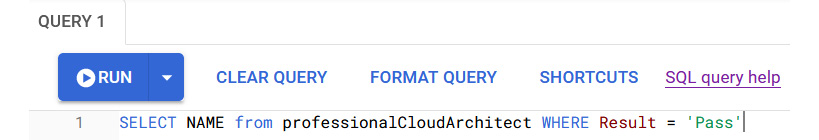
   Figure 12.8 – Query

9. Let's view our results, as follows:

Figure 12.9 – Results

By doing this, we get a list of team members who have passed the exam.

IAM

Access to Google Cloud Spanner is secured with IAM. The following is a list of predefined roles, along with a short description for each:

• Spanner Admin: This person has complete rights to all Cloud Spanner resources in a project.
• Spanner Database Admin: This person has the right to list all Cloud Spanner instances and create/list/drop databases in the instances it was created in. They can grant and revoke access to a database in the project, and they can also read and write to all Cloud Spanner databases in the project.
• Spanner Database Reader: This person has the right to read from the Cloud Spanner database, execute queries on the database, and view the schema for the database.
• Spanner Database User: This person has the right to read and write to a Cloud Spanner database, execute SQL queries on the database, and view and update the schema for the database.
• Spanner Viewer: This person has the right to view all Cloud Spanner instances and view all Cloud Spanner databases.
• Restore Admin: This person has the right to restore databases from backups.
• Backup Admin: This person has the right to create, view, update, and delete backups.

Quotas and limits

Cloud Spanner comes with predefined quotas. These default quotas can be changed via the Navigation menu and via IAM & Admin | Quotas. From this menu, we can review the current quotas and request an increase for these limits. We recommend that you are aware of the limits for each service as this can have an impact on your scalability. For Cloud Spanner, we should be aware of the following limits:

• There is a limit of 2 to 64 characters on the instance ID's length.
• There is a limit of 100 databases per instance.
• There is a limit of 2 to 30 characters on the database ID's length.
• There is a limit of 2 TB storage per node.
• There is a limit of a 10 MB schema size.
• There is a limit of a 10 MB schema change size.
• There is a limit of 5,000 tables per database.
• There is a limit of 1 to 128 characters for the table name's length.
• There is a limit of 1,024 columns per table.
• There is a limit of 1 to 128 characters for the column name's length.
• There is a limit of 10 MB of data per column.
• There is a limit of 16 columns in a table key.
• There is a limit of 10,000 indexes per database.
• There is a limit of 32 indexes per table.
• There is a limit of 16 columns in an index key.
• There is a limit of 1,000 function calls.
• There is a limit of 25 nodes per project, per instance configuration.

Pricing

Cloud Spanner charges for the amount of compute capacity and the amount of storage and network bandwidth that's used. We will be charged for the following:

• For the maximum number of nodes multiplied by the hourly rate. As Spanner has moved to processing units, this might be a fraction of a full node (1,000 processing units are smaller than 1 node).
• The average amount of data in our databases over 1 month. These prices will fluctuate, depending on the location of our instances.
• Egress network traffic for some types of traffic. However, there is no charge for replication or ingress traffic.
• The amount of storage that backups use is also charged over 1 month, multiplied by the monthly rate.

  Exam Tip

  An important point to remember about Cloud Spanner is that it offers ACID transactions. If an atomic transaction involves two or more pieces of information, then all of the pieces are committed; otherwise, none are.

Bigtable

There is a clue in the name, but Bigtable is GCP's big data NoSQL database service. Bigtable is low latency and can scale to billions of rows and thousands of columns. It's also the database that powers many of Google's core services, such as Search, Analytics, Maps, and Gmail. This makes Bigtable a great choice for analytics and real-time workloads as it's designed to handle massive workloads at low latency and high throughput.

Exam Tip

Bigtable can support petabytes of data and is suitable for real-time access and analytics workloads. It's a great choice for Internet of Things (IoT) applications that require frequent data ingestion or high-speed transactions.

Given Bigtable's massive scalability, we will cover the storage model and architecture. When we discuss Bigtable, we will make references to HBase. HBase is effectively an open source implementation of the Bigtable architecture and follows the same design philosophies. Bigtable stores its data in tables, which are stored in a key/value map. Each table is comprised of rows, which will describe a single entity.

Tables are also comprised of columns, which contain individual values for each row. Rows are indexed by a row key, and columns that are related to one another are grouped into a column family. Bigtable only offers basic operations such as create, read, update, and delete. This means it has some good use cases while also not being great for others. Bigtable should not be used for transaction support – as we mentioned previously, CloudSQL or Spanner would be better suited for OLTP.

The following diagram shows the architecture of Bigtable:

Figure 12.10 – Bigtable architecture

Here, we can see that the client's requests go through a frontend server before they are sent to a Bigtable node. These nodes make up a Bigtable cluster belonging to a Bigtable instance, which acts as a container for the cluster.

Each node in the cluster handles a subset of the requests. We can increase the number of simultaneous requests a cluster can handle by adding more nodes. The preceding diagram only shows a single cluster, but replication can be enabled by adding a second cluster. With a second cluster, we can send different types of traffic to specific clusters and, of course, availability is increased.

To help balance out the workload of queries, Bigtable is sharded into blocks on contiguous rows. These are referred to as tablets and are stored on Google's filesystem – Colossus – in Sorted Strings Table (SSTable) format. SSTable stores immutable row fragments in a sorted order based on row keys. Each table will be associated with a specific Bigtable node, and writes are stored in the Colossus shared log as soon as they have been acknowledged. We should also note that data is never stored on Bigtable nodes. However, these nodes have pointers to a set of tablets that are stored in Colossus, meaning that if a Bigtable node fails, then no data loss is suffered.

Now that we understand the high-level architecture, let's look at the configuration of Bigtable.

Bigtable configuration

In this section, we will look at the key components that make up Bigtable. We will discuss the following:

• Instances
• Clusters
• Nodes
• Schema
• Replication

Instances

Cloud Bigtable is made up of instances that will contain up to four clusters that our applications can connect to. Each cluster contains nodes. We should imagine an instance as a container for our clusters and nodes. We can modify the number of nodes in our cluster and the number of clusters in our instance. When we create our instance, as expected, we can select the region and zone that we wish to deploy to and we can also select the type of storage, either SSD or HDD. The location and the storage type are both permanent choices.

Clusters

A Bigtable cluster represents the service in a specific location. Each cluster belongs to a single Bigtable instance and, as we've already mentioned, each instance can have up to four clusters. When our application sends a request to an instance, it is handled by one of the clusters in the instance. Each cluster is located in a single zone, and an instance's clusters must be in unique zones. If our configuration means that we have more than one cluster, then Bigtable will automatically start to replicate our data by storing copies of the data in each of the cluster's zones and synchronizing updates between the copies. To isolate different types of traffic from each other, we can select which cluster we want our application to connect to.

Nodes

Each cluster in a production instance has a minimum of three nodes. Nodes are, as you may expect, compute resources that Bigtable will use to manage our data. Bigtable will try to distribute read and writes evenly across all nodes and also store an equal amount of data on each node. If a Bigtable cluster becomes overloaded, we can add more nodes to improve its performance. Equally, we can scale down and remove nodes.

Schema

It's worth noting that designing a Bigtable schema is very different from designing a schema for a relational database. There are no secondary indices as each table only has one index. Rows are sorted lexicographically by row key (the only index), from the lowest to the highest byte string. If you have two rows in a table, one row may be updated successfully while the other row may fail. Therefore, we should avoid designing schemas that require atomicity across rows. Poor schema designs can be responsible for overall poor Bigtable performance.

Exam Tip

Schemas can also be designed for time series data. If we want to measure something along with the time it occurred, then we are building a time series. Data in Bigtable is stored as unstructured columns in rows, with each row having a row key. This makes Bigtable an ideal fit for time series data. When we have to think about schema design patterns for time series, we should use tall and narrow tables, meaning that one event is stored per row. This makes it easier to run queries against our data.

Replication

The availability of data is a very big concern. Bigtable replication copies our data across multiple regions or zones within the same region, thus increasing the availability and durability of our data. Of course, to use replication, we must create an instance with more than one cluster or add clusters to an existing instance. Once this has been set up, Bigtable will begin to replicate straight away and store separate copies of our data in each zone where our instance has a cluster. Since this replication is done in almost real time, it makes for a good backup of our data. Bigtable will perform an automated failover when a cluster becomes unresponsive.

Application profiles

If we require an instance to use replication, then we need to use application profiles. By storing settings in these application profiles, we can manage incoming requests from our application and determine how Bigtable handles them. Every Bigtable instance will have a default application profile, but we can also create custom profiles. Our code should be updated to specify which app profile we want our applications to use when we connect to an instance. If we do not specify anything, then Bigtable will use the default profile.

The configuration of our application profiles will affect how an application communicates with an instance that uses replication. There are routing policies within an application profile. Single-cluster routing will route all the requests to a single cluster in your instance, while multi-cluster routing will automatically route traffic to the nearest cluster in an instance. If we create an instance with one cluster, then the default application profile will use single-cluster routing. If we create an instance with two or more clusters, then the default application profile will use multi-cluster routing.

To create an application profile, we must have a Bigtable instance. We can create a custom application profile from the GCP console by browsing to the hamburger menu and going to Bigtable, and then clicking on the instance where we wish to create the app profile. Finally, browse to the Application profiles option in the left-hand pane and click CREATE APPLICATION PROFILE.

In the following screenshot, we are creating an application profile for an instance called cloudarchitect:

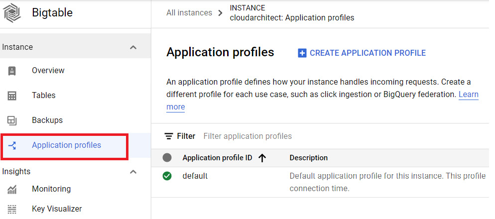
Figure 12.11 – Application profiles

Then, we need to give the profile an ID and enter a description if we feel that's necessary. Afterward, we must select the routing policy we require:

Figure 12.12 – Application profile settings

Note that we can check the box for single-row transactions. Bigtable does not support transactions that atomically update more than one row; however, it can use single-row transactions to complete read-modify-write and conditional writes operations. Note that this option is only available when using a single-cluster routing policy to prevent conflicts.

Data consistency

One important aspect to understand is that Bigtable is eventually consistent by default, meaning that when we write a change to one of our clusters, we will be able to read that change from other clusters, but only after replication has taken place. To overcome this constraint, we can enable Read-Your-Writes consistency when we have replication enabled. This will ensure that an application won't read data that's older than the most recent writes. To achieve Read-Your-Writes consistency for a group of applications, we should use the single-cluster routing policy in our app profiles to route requests to the same cluster. The downside to this, however, means that if a cluster becomes unavailable, then we need to perform the failover manually.

Planning capacity

One important aspect to consider when planning our Bigtable clusters is the trade-off between throughput and latency. For latency-sensitive applications, Google advises that we plan for at least 2x capacity for our application's maximum Bigtable QPS. This is to ensure that Bigtable clusters run at less than 50% CPU usage, therefore offering low latency to frontend services.

Exam Tip

Capacity planning allows us to provide a buffer for traffic spikes or key-access hotspots, which may cause imbalanced traffic among nodes in the cluster.

Creating a Bigtable instance and table

Let's take a look at creating a Bigtable instance from our GCP console:

1. Browse to DATABASES | Bigtable, as shown in the following screenshot:
   

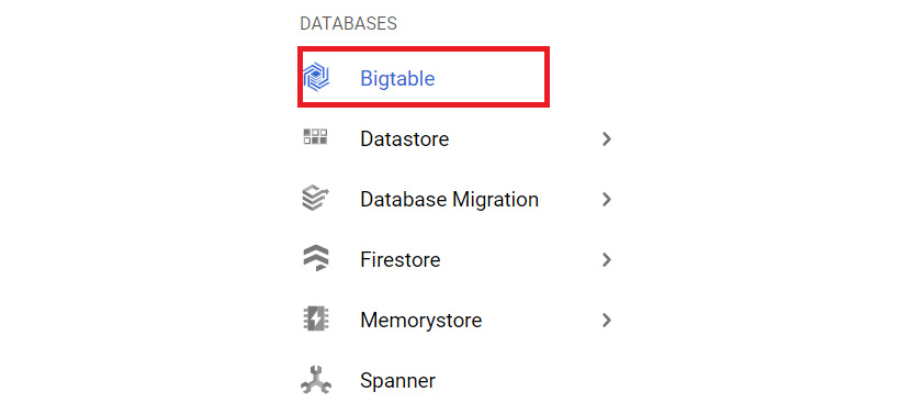
   Figure 12.13 – Bigtable

2. Click on CREATE INSTANCE:
   

   Figure 12.14 – Creating an instance

3. Provide a name and instance ID for our instance and select an instance type. Also, select the type of storage we require:
   

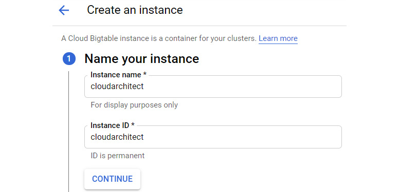
   Figure 12.15 – Instance configuration

4. Provide the cluster details; that is, the location and the number of nodes needed. We can also set up replication if needed. Note that we can also select our storage type – either SSD or HDD. This will default to SSD if we do not change it. Click Done to accept the cluster changes and click Create to complete the instance configuration:

Figure 12.16 – Adding a cluster

Once we have our instance and clusters, we can create a table. We touched on this earlier, but Bigtable has a command-line tool called cbt, and creating a table is simplistic when we use it. Once again, we will make assumptions that you are familiar with this tool. Open Cloud Shell so that we can configure the cbt tool. We will look at cbt and Cloud Shell in more detail in Chapter 16, Google Cloud Management Options:

1. Before we create a table, run the following syntax to mitigate the need to specify them in future command lines:

   echo project = <project ID> ~/.cbtrc

   echo instance = <instance ID> >> ~/.cbtrc

   Here, we have the following:

   • <project ID> is the ID of the project our Bigtable instance is associated with.
   • <instance ID> is the ID of our instance.
2. Once this has been configured, we can create a table using some very simple syntax:

   cbt createtable table001

Here, we have created a table called table001.

IAM

Access to Google Cloud Bigtable is secured with IAM. The following is a list of predefined roles, along with a short description of each:

• Bigtable Admin: This person has rights to all Bigtable features and is where you can create new instances. This role should be used by project administrators.
• Bigtable User: This person has read-only access to the data stored within tables. This role should be used by application developers or service accounts.
• Bigtable Reader: This person has read-only access to the data stored within tables. This role should be used by data scientists.
• Bigtable Viewer: This role should be used to grant the minimal set of permissions for Cloud Bigtable.

Quotas and limits

Google Cloud Bigtable comes with predefined quotas. These default quotas can be changed via the Navigation menu and via IAM & Admin | Quotas. From this menu, we can review the current quotas and request an increase for these limits. We recommend that you are aware of the limits for each service as this can have an impact on your scalability. For Cloud Bigtable, we should be aware of the following limits:

• There is a limit of 2.5 TB of SSD storage per node.
• There is a limit of 8 TB of HDD storage per node.
• There is a limit of 1,000 tables in each instance.

For Cloud Bigtable, we should also be aware of the following quotas:

• By default, you can provision up to 30 SSD or HDD nodes per zone in each project.
• Numerous operational quotas should be reviewed.

Pricing

Bigtable charges based on several factors:

• Instance types are charged per hour, per node.
• Storage is charged per month and costs vary, depending on the use of SSD or HDD.
• Internet egress rates are charged depending on monthly usage. Ingress traffic is free.

For more specific details, please see the Bigtable pricing URL in the Further reading section.

Summary

In this chapter, we covered Cloud Spanner and Bigtable.

In terms of Cloud Spanner, we now understand that this is a scalable and globally distributed database. It is strongly consistent and was built to combine the benefits of relational databases with the scalability of a non-relational database. Cloud Spanner can scale across regions for workloads that might have high availability requirements.

We covered Bigtable at a high level to make sure you are aware of what is expected in the exam. It is a fully managed NoSQL database service that can scale massively and offers low latency, is ideal for IoT as it can handle high-speed transactions in real time, integrates well with machine learning and analytics, and can support over a petabyte of data.

We have now come to the end of a large chapter with a lot of information to take in. We have looked at the key database services offered by GCP. We advise that you look over the exam tips in this chapter and make sure that you are aware of the main features of each service. Some of the key design decisions that we have spoken about are relational versus non-relational, structured data versus non-structured data, scalability, and SQL versus NoSQL.

In the next chapter, we will look at big data.

Further reading

Read the following articles to find out more about what was covered in this chapter:

• Cloud Spanner: https://cloud.google.com/spanner/docs/
• Cloud Spanner Pricing: https://cloud.google.com/spanner/pricing
• Bigtable: https://cloud.google.com/Bigtable/docs/
• Bigtable Pricing: https://cloud.google.com/Bigtable/pricing