Chapter 5: Splitting the Model

In this chapter, we will discuss how to train giant models with model parallelism. Giant models refers to models that are too large to fit into a single GPU's memory. Some examples of giant models include Bidirectional Encoder Representations from Transformers (BERT), Generative Pre-Trainer Transformer (GPT): GPT-2 and GPT-3.

In contrast to data parallel workloads, model parallelism is often adopted for language models. Language models are a specific type of deep learning model that works in the Natural Language Processing (NLP) domain. Here, the input data is usually text sequences. The model outputs predictions for tasks such as question answering and next sentence prediction.

NLP model training is often segregated into two different types, pre-training and fine-tuning. Pre-training means training the whole giant model from scratch, which may need a huge amount of data and plenty of training epochs. Fine-tuning uses pre-trained models as the base model. We can then fine-tune the base model on some specific downstream tasks. Thus, fine-tuning usually takes much less time to train than pre-training. Also, a fine-tuning dataset is much smaller compared to a pre-training dataset.

Some general assumptions for this chapter are listed as follows:

• For each NLP training job, we usually focus on the fine-tuning process and not the pre-training process.
• For the fine-tuning process, we use a much smaller training dataset than the training data used in the pre-training process.
• We assume each job ran exclusively on a set of GPUs or other accelerators.
• We assume a model has enough layers to split across multiple GPUs.
• We assume we always have a pre-trained model available for fine-tuning.

In this chapter, we will first explain why model parallelism is important by pointing out that single-node training for giant models can cause out-of-memory errors on accelerators. Second, we will briefly discuss several representative NLP models, given that people may not be familiar with these giant models if they have never tried model-parallel training. Third, we will discuss two separate training stages of using pre-trained giant models. Finally, we will explore some state-of-the-art hardware for training these giant models.

In summary, you will learn the following topics in this chapter:

• Single-node training error – out of memory
• ELMo, BERT, and GPT
• Pre-training and fine-tuning
• State-of-the-art hardware

Technical requirements

For the implementation in the rest of the sections, we may illustrate it in BERT or GPT models. We will use the Stanford Question Answering Dataset (SQuAD 2.0) as our dataset. We will also use PyTorch for illustration. The main library dependencies for our code are as follows:

• torch>=1.7.1
• transformers>=4.10.3
• cuda>=11.0
• NVIDIA driver>=450.119.03

It is mandatory to have the preceding libraries pre-installed with their correct versions.

Dataset Citation

SQuAD: 100,000+ Questions for Machine Comprehension of Text, Pranav Rajpurkar, Jian Zhang, Konstantin Lopyrev, and Percy Liang, arXiv preprint arXiv:1606.05250 (2016): https://rajpurkar.github.io/SQuAD-explorer/.

Single-node training error – out of memory

Giant NLP models, such as BERT, are often hard to train using a single GPU (that is, single-node). The main reason is due to the limited on-device memory size.

Here, we will first fine-tune the BERT model using a single GPU. The dataset we will use is SQuAD 2.0. It often throws an Out-of-Memory (OOM) error due to the giant model size and huge intermediate results size.

Second, we will use a state-of-the-art GPU and try our best to pack the relatively small BERT-base model inside a single GPU. Then, we will carefully adjust the batch size to avoid an OOM error.

Fine-tuning BERT on a single GPU

The first thing we need to do is to install the transformers library on our machine. Here, we use the transformers library provided by Hugging Face. The following command is how we install it on an Ubuntu machine using PyTorch:

$ pip install transformers

Please make sure you are installing the correct transformers version (>=4.10.3) by double-checking, as follows:

Figure 5.1 – Checking the transformers version

Then, we can start using the pre-trained model for our fine-tuning tasks.

We will illustrate how to implement the training process in the later sections. Now, assuming we have successfully started the training job, it prints out the following error messages:

Figure 5.2 – Error messages

The preceding error messages indicate that the training job has run OOM on the GPUs. It indicates that a single GPU is not enough for holding a giant model and gives some intermediate results from the inputs.

A Single GPU Training Giant NLP Models

Using a single GPU to train a giant NLP model will cause an OOM error. The main reason for this is that the model parameter size is too large. Consequently, the intermediate results generated from the input are also very large.

Given this OOM error, it is natural to think about splitting the model and spreading the model partitions across different GPUs. This is what we call model parallelism.

Model Parallelism

Model parallelism works by taking the following two steps:

1. Splitting the model weights into a disjoint subset

2. Spreading each model partition onto a single accelerator

Before we dive into model parallelism, we will first try to use one state-of-the-art GPU, NVIDIA V100, to pack a relatively small BERT model into a single GPU. We will discuss the pros and cons of doing this in the following section.

Trying to pack a giant model inside one state-of-the-art GPU

Here, we will try to use a state-of-the-art GPU, which is NVIDIA V100. The following figure shows the technical specifications of a V100 GPU:

Figure 5.3 – Technical specifications of a V100 GPU

As shown in the preceding figure, a V100 GPU has 16160MiB (~16 GB) of on-device memory. The peak power consumption can be 300W. This is one of the GPUs that has the largest on-device memory size.

Now, let's try to pack a BERT-base model into this single V100 GPU.

Before the training starts, we need to preprocess the input data, which is as follows:

Figure 5.4 – Preprocessing the input data

After we generate the training samples, we launch our training job.

To fit into a single GPU's memory, here we use a very small batch size of four. The following is the system information on fine-tuning BERT with the SQuAD 2.0 dataset:

Figure 5.5 – System information on fine-tuning BERT with the SQuAD 2.0 dataset

As shown in the preceding figure, with a batch size of four, the BERT-based model can be trained inside a single V100 GPU. However, when you look at the computation core utility rate (that is, Volatile GPU-Util in the preceding figure), it is just around 83%. This means around 17% of computation cores are wasted.

Note that this volatile GPU-Util rate is a coarse metric, which means that the real GPU core usage is usually even lower than the number that is shown here.

We will also test another extreme case with a batch size of one. The following is the GPU utility status:

Figure 5.6 – Testing with the batch size as one – GPU utility status

As shown in the preceding figure, the GPU utility in this case is just 65%, which means almost half of the GPU core is wasted during training. One thing worth mentioning is that the training time can be insanely long if we just use a tiny batch size such as one or four.

Another thing is, right now, we only test relatively small models as BERT-base. With some other bigger models, such as BERT-large, GPT-3 is not possible to fit into a single GPU's memory.

To sum up, single-node training often causes an OOM error when training giant NLP models.

Even in some extreme cases, we can pack a relatively small NLP model inside a single GPU. However, it may not be practical due to the following reasons:

• Local training batch size is too small; thus the overall training time will be insanely long.
• A small batch size also leads to the wastage of computation cores.

Next, we will discuss common NLP models used nowadays.

ELMo, BERT, and GPT

In this section, we will explain several classic NLP models used nowadays, namely ELMo, BERT, and GPT.

Before we dive into these complicated model structures, we will first illustrate the basic concept of a Recurrent Neural Network (RNN) and how it works. Then, we will move on to the transformers. This section will cover the following topics:

• Basic concepts
• RNN
• ELMo
• BERT
• GPT

We will start with introducing RNNs.

Basic concepts

Here, we will dive into the world of RNNs. At a high-level, different from CNNs, an RNN usually needs to maintain the states from previous input. It is just like memory for human beings.

We will illustrate what we mean with the following examples:

Figure 5.7 – One-to-one problems

As shown in the preceding figure, one-to-one is a typical problem format in the computer vision domain. Basically, assuming we have a CNN model, we input an image as Input 1, as shown in Figure 5.7. The CNN model will output a prediction value (for example, an image label) as Output 1 in Figure 5.7. This is what we call one-to-one problems.

Next, we will discuss one-to-many problems, as illustrated in Figure 5.8:

Figure 5.8 – One-to-many problems

What's shown in the preceding figure is another typical task, called a one-to-many problem. It is one of several common tasks for an NLP model, for example, image captioning. We can input an image and the model produces the output as a sentence describing what is inside the image.

It is worth mentioning that models 1, 2, and 3 are the same models as in Figure 5.8. The only difference is that Model 2 received some states information from Model 1, and Model 3 received some states memory from Model 2.

Next, we will discuss many-to-one problems, as shown in the following figure:

Figure 5.9 – Many-to-one problems

There is another kind of workload that requires an RNN-based model. It is called a many-to-one problem.

Basically, we are given a sequence of inputs (for example, a sentence with multiple words). After processing each word in a sequential order, we output one value. One example of a many-to-one problem would be sentiment classification. For example, after reading a sentence from a customer review, the model predicts whether it is a positive comment or a negative one.

Next is a many-to-many problem. We have two sub-categories in this setting, which are shown in Figure 5.10 and Figure 5.11 respectively:

Figure 5.10 – Many-to-many problems (no delay)

The first type of many-to-many problem is the no-delay version. This means that, after getting one input, the model will immediately predict one output. As shown in the preceding figure, there is no delay between Input 1 and Output 1, or Input 2 and Output 2.

A common application is video classification and motion capturing. Basically, for each frame of the input image, we need to tag the objects in the picture and monitor their movements.

Next, we will discuss another many-to-many problem with delay, as shown in the following figure:

Figure 5.11 – Many-to-many problems (with delay)

As shown in the preceding figure, the second version of a many-to-many problem is having a delay between the input and output. As shown in the preceding figure, Output 1 will not be generated until we pass in Input 2. This is the reason we call it a many-to-many problem with delay.

One typical example of this is machine translation. Basically, once we get the first word of a sentence from language A, we wait and collect more words from the input sentence, and then we provide the output as the translation of the sentence from language A to language B.

RNN

Apart from the one-to-one problem defined in the preceding section, all other problems have some dependency on previous states. For example, in Figure 5.11, in order to get Model 2 weights, we need Model 1 to memorize some information from Input 1 and pass this information to Model 2.

Although Model 1 and Model 2 are the same models, they maintain different intermediate states. For example, in Figure 5.11, Model 2's state maintains information from both Model 1 and Input 2.

To pass state information within the same model, we define some recurrent links on the model. A model with a recurrent link is called an RNN, shown in the following figure:

Figure 5.12 – RNN structure

As shown in the preceding figure, the main difference between an RNN and other models such as a CNN is that an RNN has a recurrent link within the model itself.

This recurrent link is used for maintaining input-related states inside the model. For example, when the model receives the second input, it can use both the first input's states and the second input to predict the output.

An unrolled version of an RNN is shown in the following figure. Here, we unroll the RNN in the time dimension:

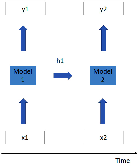
Figure 5.13 – Unrolled RNN structure over time

As shown in the preceding figure, at the first time slot, after the model processes input 1 (that is, x1), it will generate output 1 (that is, y1). At the same time, it will maintain some hidden states (for example, h1 stands for hidden state at time 1).

At the second time slot, the model will receive input 2. Here, the model will do two things, as follows:

1. Calculate the new hidden state, as follows:

Here, Wh is the model's weight for memorizing hidden information such as h1, h2 ... ht. Wx is the weight matrix for current input, such as x2, x3, ... xt. For most DNN models, we also need to add bias at the very end of the calculation.

Basically, to calculate the new hidden state h2, we need to aggregate the previous hidden state and current input data.

2. Use the new hidden state h2 and x2 to generate the output y2, as follows:

To calculate the output at time slot 2 (that is, y2 in Figure 5.13), we need to use the updated hidden state h2 and weight matrix for output (that is, Wy). Similarly, we add the bias item at the end of this equation.

With the preceding two equations, at any given time i we can do the following:

1. Update the hidden state h[i] with the previous hidden state h[i-1] and current input x[i].
2. Then, use the updated h[i] to generate the current output y[i].

These are the key concepts regarding the simplest NLP model, which is an RNN. In a real-world application, we usually stack an RNN as shown in the following figure:

Figure 5.14 – Stacked RNN (deep RNN)

In the preceding figure, we illustrate a simplified stacked RNN that stacks two RNNs together.

You may regard Layer 1 as the RNN we described in Figure 5.13. On top of that, we stack another RNN called Layer 2.

Basically, for one particular layer of the stacked RNN, the following applies:

• It takes the previous RNN layer's output as its own input.
• After generating its own output, it passes the output to its successive RNN layer as the input.

It is common that a stacked RNN has a better test accuracy compared with a single-layer RNN. Thus, for a real-world application, a stacked RNN is often a better choice.

ELMo

ELMo is a special kind of RNN. It is based on Long Short-Term Memory (LSTM).

LSTM can be regarded as a complicated version of the RNN we mentioned in the previous section. Basically, each LSTM cell has a multiple-gating system for maintaining both long-term and short-term memory of the data.

In a traditional RNN, the hidden state is always propagated in the same order as the input sequence. In the following figure, for Layer 1, the hidden state is passed as h1_1 and then h1_2, which is the same order as inputs x1 and x2:

Figure 5.15 – Forward part of the ELMo model

In contrast to a traditional RNN model, ELMo actually maintains another model that backward-propagates hidden states, as seen in the following figure:

Figure 5.16 – Backward part of the ELMo model

As shown in the preceding figure, ELMo maintains one additional model that backward-propagates the hidden states information. For example, for Layer 1, the hidden state is propagated from hb1_2 to hb1_1, which is the inverse order of x1, x2, and x3.

Since ELMo maintains two model parts, one forward-propagates the hidden states and the other backward-propagates the hidden states. Thus, for each input, for a layer, we may have two different hidden states.

For example, in Figure 5.15 and Figure 5.16, for x2 Layer 1 has a forward hidden state as h1_1 and a backward hidden state as hb1_2. ELMo will use both hidden states to represent x2.

Therefore, in ELMo, for a particular input, we have two groups of hidden states, one a group of forward hidden states and the other a group of backward hidden states. This decent feature guarantees that ELMo can learn the input relationship in both forward and backward directions. This richer information contributes to the higher test accuracy of ELMo when comparing with forward-only RNN models.

We have just discussed all the classical models using an RNN. Next, we will discuss transformer-based models, such as BERT and GPT-2/3.

BERT

The BERT model was invented by Google. The base component of the BERT model is the transformer.

A transformer adopts a similar idea to ELMo's bidirectional training. However, a transformer extends it one step further by adopting self-attention. A simplified self-attention unit is shown in the following figure:

Figure 5.17 – Simplified self-attention

We use the same example as Figure 5.12. Let's assume we have a single-layer model, and we want to calculate the output o1 given the input x1. In a self-attention scheme, it removes the direct hidden state, passing links as h1_1 or hb1_1 as we saw in Figure 5.15 and Figure 5.16 respectively. Instead, self-attention uses all the memory information from all the input tokens (for example, x1, x2, and x3 in Figure 5.17) together.

For example, in order to calculate o1 in Figure 5.17, self-attention defines the correlation of x1 with all input tokens (that is, x1, x2, and x3). It works in two steps:

1. We regard the correlation as a weight matrix, such as w1, w2, and w3 in Figure 5.17.
2. Then, we use both correlation matrices and some values generated from each input (that is, v1, v2, and v3) together to calculate output o1.

The formal definition for calculating o1 is as follows:

For other output such as o2 and o3, it follows the preceding equation as well.

At a high level, the main difference between a bidirectional RNN and self-attention is as follows:

• In a bidirectional RNN (such as ELMo), the hidden state for one input token only depends on its previous or successive input states.
• In self-attention, the intermediate representation of one input token depends on all the input tokens together.

In reality, a transformer uses multi-head attention, which is to calculate multiple attention output values for each input.

For example, for the o1 case mentioned previously, multi-head attention will calculate o1_1, o1_2, and so on. Each o1_i has different correlation matrices such as w1_i, w2_i, w3_i, and so on.

BERT borrows the bidirectional transformer concepts and stacks multiple layers of bidirectional transformers together, as shown in the following figure:

Figure 5.18 – A simplified BERT model

The preceding figure shows a simplified BERT model illustration. We stack two bidirectional transformer layers. Here, a bidirectional transformer refers to the attention values for each input that not only depend on all its previous input tokens but also its successive input tokens.

Next, we will discuss GPT, a slightly different transformer-based NLP model.

GPT

A GPT model was developed by OpenAI, which is also a transformer-based NLP model. Currently, the most popular types of GPT models are GPT-2 and GPT-3. Both GPT-2 and GPT-3 are giant models. The commonly used model versions are not able to fit into a single GPU's memory.

Compared with BERT, GPT models adopt a slightly different transformer as the base components. A simplified structure for a GPT model is shown here:

Figure 5.19 – A simplified GPT model

As shown in the preceding figure, the transformer layer here is slightly different than the one in Figure 5.18.

Here, each input's attention value only depends on its previous input tokens and is not related to its successive input tokens. Thus, we call it a one-directional transformer or forward-only transformer, while we call the BERT-version transformer shown in Figure 5.18 a bidirectional transformer.

Next, we will discuss two types of NLP model training.

Pre-training and fine-tuning

There are two stages in NLP models that can be described as training. One is pre-training and the other is fine-tuning. In this section, we will discuss the main difference between these two concepts.

Pre-training is where we train a giant NLP model from scratch. In pre-training, we need to have a huge training dataset (for example, all the Wikipedia pages). It works as follows:

1. We initialize the model weights.
2. We partition the giant model into hundreds or thousands of GPUs via model parallelism.
3. We feed the huge training dataset into the model-parallel training pipeline and train for several weeks or months.
4. Once the model is converged to a good local minimum, we stop the training and call the model a pre-trained model.

By following the preceding steps, we can get a pre-trained NLP model.

Note that the pre-training process often takes huge amounts of computational resources and time. As of now, only big companies such as Google and Microsoft have the resources to pre-train a model. Pre-training is rarely seen in academia.

Fine-tuning is to slightly adjust the pre-trained model with different downstream tasks. For example, a BERT model is pre-trained for tasks such as the following:

• Masked language modeling
• Next sentence prediction

However, you can also use BERT for other tasks, such as the following:

• Question answering
• Sequence classification

You need to fine-tune the pre-trained BERT model for these new downstream tasks.

Suppose you train the pre-trained BERT model for question answering. You need to fine-tune the pre-trained BERT model on a much smaller question-answering dataset, such as SQuAD 2.0.

One thing worth mentioning is that, compared to pre-training, the fine-tuning process often takes much less computational resources and costs less training time. In addition, fine-tuning is often training the pre-trained model on some small datasets.

Pre-Training versus Fine-Tuning

Pre-training is when you train a model from scratch.

Fine-tuning is when you adjust the pre-trained model weights with new downstream tasks.

Since most of the NLP models are giant, we often use the best GPUs to train these models concurrently. Next, we will discuss state-of-the-art hardware. We will mainly focus on discussing the GPUs from NVIDIA.

State-of-the-art hardware

Due to the huge computation power needed for training giant NLP models, we usually use a state-of-the-art hardware accelerator to do the NLP model training. In the following sections, we will look into some of the best GPUs and hardware links from NVIDIA.

P100, V100, and DGX-1

Tesla P100 GPU and Volta V100 GPU are the best GPUs launched by NVIDIA. Each P100/V100 GPU has the following:

• 5–8 teraflops of double-precision computation power
• 16 GB on-device memory
• 700 GB/s high bandwidth memory I/O
• NVLink-optimized

As per the specification listed in the preceding list, each P100/V100 GPU has a huge amount of computation power. There is an even more powerful machine that includes eight P100/V100 GPUs inside a single box. The eight-P100/V100-GPU box is called DGX-1.

DGX-1 is designed for high-performance computation. When embedding eight P100/V100 GPUs inside a single box, the cross-GPU network bandwidth becomes the main bottleneck during in-parallel model training.

Therefore, DGX-1 introduces a new hardware link called NVLink.

NVLink

NVLink is a GPU-exclusive, point-to-point communication link among GPUs inside one DGX-1 box.

NVLink can be regarded as a much faster PCIe bus but only connects with GPUs. PCIe 3.0 communication bandwidth is around 10 GB/s. Compared with PCIe, each NVLink can provide around 20–25 GB/s of communication bandwidth among GPUs.

In addition, for the P100 version, the NVLink among the GPUs within a DGX-1 machine forms a special hyper-cube topology, which is shown in Figure 5.20.

As shown in Figure 5.20, we have two different four-GPU islands. G0–G3 forms one island and G4–G7 forms another island. The hyper-cube topology has the following attributes:

• Within one island, the four GPUs are fully connected.
• Between two islands, only counterpart GPUs are connected (for example, G0–G4 and G2–G6).

The following figure shows the hyper-cube topology:

Figure 5.20 – Hyper-cube NVLink topology inside a DGX-1 machine

For DGX-1 with eight V100 GPUs, the NVLink topology looks similar to the preceding figure. More specifically, besides the hyper-cube topology in Figure 5.20, DGX-1 (with V100) adds an additional NVLink ring that connects G0, G3, G2, G6, G7, G4, G5, and G1.

A100 and DGX-2

Currently, the best GPU from NVIDIA is called A100. The following are some of the main specifications of A100:

• 10 teraflops of double-precision computation power
• 40 GB on-device memory
• 1,500 GB/s memory bandwidth
• NVSwitch-optimized

The DGX-2 machine packs 16 A100 GPUs inside a single box. These 16 A100s are connected by NVSwitch.

NVSwitch

NVSwitch is the new generation of cross-GPU communication channels. It can be regarded as a switch in computer networks that enables point-to-point communication bandwidth of 150 GB/s unidirectionally and 300 GB/s bidirectionally among GPUs.

Summary

In this chapter, we mainly discussed NLP models and state-of-the-art hardware accelerators. After reading this chapter, you now understand why NLP models are usually not suitable to be trained on a single GPU. You also now know basic concepts such as the structure of an RNN model, a stacked RNN model, ELMo, BERT, and GPT.

Regarding hardware, you now know about several state-of-the-art GPUs from NVIDIA and the high-bandwidth links in between.

In the next chapter, we will cover the details of model parallelism and some techniques to improve system efficiency.