Chapter 6: Pipeline Input and Layer Split

In this chapter, we will continue our discussion about model parallelism. Compared to data parallelism, model parallelism training often takes more GPUs/accelerators. Thus, system efficiency plays an important role during model parallelism training and inference.

We limit our discussion with the following assumptions:

• We assume the input data batches are the same size.
• In multi-layer perceptrons (MLPs), we assume they can be calculated with general matrix multiply (GEMM) functions.
• For each NLP job, we run it exclusively over a set of accelerators (for example, GPUs). This means there is no interference from other jobs.
• For each NLP job, we use the same type of accelerator (for example, GPUs).
• GPUs within a machine are connected with homogeneous links (for example, NVLink or PCIe).
• For cross-machine communication, the machines are also connected with homogeneous links (for example, an Ethernet cable).
• For model parallelism training, we are focusing on fine-tuning. Thus, we assume we have a pre-trained NLP model.
• For each input batch, the number of items is large enough to be split into multiple partitions.
• For each layer of the model, there are enough neurons for us to split and re-distribute them to multiple accelerators.
• For the number of layers of an NLP model, there are enough layers for us to partition them among multiple accelerators.

In this chapter, we will mainly focus on system efficiency in model parallelism. First, we will discuss the shortcomings of vanilla model parallelism. Vanilla model parallelism cannot scale well mainly due to system inefficiency. Second, we will cover the first kind of approach (pipeline parallelism) to improve system efficiency in model parallelism training. Third, we then describe pipeline parallelism on top of model parallelism in order to improve system efficiency. Fourth, we will discuss the advantages and disadvantages of using pipeline parallelism. Fifth, we will discuss a second kind of approach, that is, intra-layer model parallelism. And lastly, we will discuss variations of intra-layer model parallelism.

In summary, we will cover the following topics in this chapter:

• Vanilla model parallelism is inefficient
• Pipeline parallelism
• Pros and cons of pipeline parallelism
• Layer split
• Notes on intra-layer model parallelism

Now we will illustrate why vanilla model parallelism is very inefficient. Then we will discuss pipeline parallelism and intra-layer model parallelism separately.

Vanilla model parallelism is inefficient

As mentioned in a huge number of papers from academia and technical reports from the industry, vanilla model parallelism is very inefficient regarding GPU computation and memory utilization. To illustrate why vanilla model parallelism is not efficient, let's look at a simple DNN model, which is shown in Figure 6.1:

Figure 6.1 – A simple NLP model with three layers

As shown in Figure 6.1, given the training input, we pass it into our three-layer NLP model. The layers are denoted as Layer 1, Layer 2, and Layer 3. After the forward propagation, the model will generate some output.

Now let's assume we use three GPUs. Each GPU only holds one layer of the original model. It is shown in Figure 6.2:

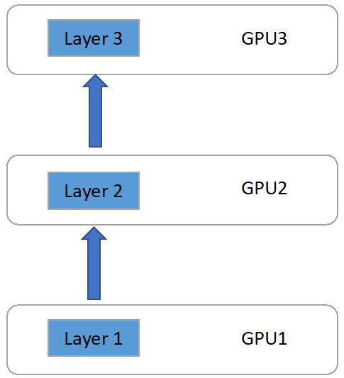
Figure 6.2 – Model partition on three GPUs

In Figure 6.2, we have GPU1 holding Layer 1 of the model. Similarly, we have GPU2 holding Layer 2 and GPU3 holding Layer 3.

Now, we will discuss forward propagation and backward propagation step by step.

Forward propagation

Given a batch of input training data, we will first conduct forward propagation on the model. Since we partition the model onto GPUs 1-3, the forward propagation happens in the following order:

1. GPU1 will first conduct forward propagation of Layer 1 on input data.
2. Then, GPU2 will start forward propagation.
3. Finally, GPU3 will start forward propagation.

The preceding three-step forward propagation can be visualized as follows:

Figure 6.3 – Forward propagation in model parallelism

As shown in Figure 6.3, on GPU1 we conduct Layer 1's forward propagation, and we rename it F1. Similarly, Layer 2's forward propagation is called F2 and Layer 3's forward propagation is called F3.

After Layer 3 is finished with forward propagation, it will generate the model's output. The model serving stage is the end of model serving for the current input data batch. However, if you are doing model training (that is, the fine-tuning stage of NLP model training), we need to generate gradients for each layer via backward propagation.

Backward propagation

After Layer 3's forward propagation (that is, F3 in Figure 6.3), it generates an output prediction. At the model parallel training stage, we compare the prediction with the correct label/output via the loss function. Then we start the backward propagation, which is illustrated in the following diagram:

Figure 6.4 – Backward propagation in model parallelism training

As shown in the preceding diagram, compared to forward propagation in Figure 6.3, backward propagation is in the reverse order. It works as follows:

1. First, Layer 3 on GPU3 starts backward propagation to generate local gradients of Layer 3. We call this Layer 3 backward propagation B3 in the preceding diagram. Then, GPU3 will pass Layer 3's gradient output to Layer 2 on GPU2.
2. After receiving GPU3's gradient output, GPU2 will use it (together with the activations generated from the previous forward propagation) to generate Layer 2's local gradients. We call Layer 2's backward propagation B2 in Figure 6.4. Then, GPU2 will pass its gradient output to GPU1.
3. Finally, Layer 1 on GPU1 conducts backward propagation and generates local gradients. We call this step B1 in Figure 6.4.

After all the layers generate their local gradients, we use these gradients to update the model parameters.

In this section, we described the details of forward propagation and backward propagation in model parallelism training. Next, we will analyze the system inefficiency during each training iteration, which consists of one forward propagation and one backward propagation.

GPU idle time between forward and backward propagation

Now let's analyze a whole training iteration, which consists of one forward propagation followed by one backward propagation. We will illustrate it using the previous three-layer model training example.

The whole workflow of one training iteration is depicted in the following diagram:

Figure 6.5 – Workflow of one training iteration with model parallelism

The whole workflow of one training iteration in model parallelism is depicted in Figure 6.5. Here, F1 means Layer 1's forward propagation, which is defined in Figure 6.3. Similarly, B1 means Layer 1's backward propagation, which is defined in Figure 6.4.

The whole workflow of one training iteration shown in Figure 6.5 is as follows:

• During the forward propagation, the execution order is F1->F2->F3.
• During the backward propagation, the execution order is B3->B2->B1.

As you can see from the preceding execution order, the execution order of backward propagation is the inverse of forward propagation. The differing execution order of forward and backward propagation in model parallelism training is one of the causes of system inefficiency.

There is plenty of GPU idle time among all three GPUs in use. For example, GPU1 is idle between the processing of F1 and B1 in Figure 6.5.

In Figure 6.6, we highlight all the time periods that each GPU is idle in, which are denoted by the double-arrow lines.

Let's look at each GPU's idle time in Figure 6.6:

• GPU 1: Idle between F1 and B1
• GPU 2: Idle during the F1 period, also between the F2 and B2 period, and the B1 period
• GPU 3: Idle during the F1, F2, B2, and B1 periods

To check how much time is spent idling, let's assume that each GPU's forward and backward propagation times are the same.

Figure 6.6 – GPU idle time in one training iteration with model parallelism

As shown in Figure 6.6, we can calculate each GPU's working and idle times as follows:

• GPU1: Working in the F1 and B1 time slots, idle in the F2, F3, B3, B2 time slots
• GPU2: Working in the F2 and B2 time slots, idle in the F1, F3, B3, B1 time slots
• GPU3: Working in the F3 and B3 time slots, idle in the F1, F2, B2, B1 time slots

As per the GPU working/idle times in the preceding list, given the assumption that the forward propagation time is equal to the backward propagation time, we can conclude that every GPU works for 1/3 of the time of one training iteration, and is idle for 2/3 of the time in one training iteration. Therefore, with vanilla model parallelism training, the average GPU utilization is only around 33%, which is very low.

The main reason for this inefficiency is that GPUs with different model partitions need to wait for each other. To be more specific, in our Figure 6.6 example, we have the following:

• After the execution of F1, GPU 1 needs to wait for B2 to complete.
• GPU 2's F2 needs to wait for GPU1's F1 to complete, and GPU2's B2 needs to wait for GPU 3's B3 to complete.
• GPU3's F3 needs to wait for GPU2's F2 to complete.

This sequential layer dependency is the main reason for system inefficiency.

Vanilla Model Parallelism Training Is Inefficient

The main reason is the sequential layer dependency. Layer dependency means that GPUs with different model partitions need to wait for other GPUs' intermediate outputs.

Note that in the preceding cases we only used three GPUs. This system inefficiency can be more severe when more GPUs are involved in a model parallelism training job.

For example, let's assume we have a 10-layer deep neural network (DNN) model, and we split each layer into a single GPU. Let's still assume each layer's forward propagation and backward propagation take roughly the same amount of time. Then, for one training iteration, the total amount of time is 20 time slots: 10 for 10 layers' forward propagation, and another 10 time slots for 10 layers' backward propagation. However, each GPU only works for 2 time slots and is idle for the other 18 time slots. The two working time slots are one for its local forward propagation and the other for its local backward propagation. Therefore, each GPU's utilization rate is only 10%.

With the assumption that each GPU's forward and backward propagation take the same amount of time with N GPUs in use, we can get the following equation:

The preceding equation is similar to the 10-GPU example mentioned previously. Basically, with N GPUs in use, we need N time slots to finish the whole forward propagation of the model, and another N time slots to finish the backward propagation of the whole model. Each GPU's working time is depicted in the following equation:

Basically, each GPU only works for two time slots: one for forward propagation, and the other for backward propagation. Now, we calculate each GPU's idle time using the following equation:

For each GPU, during the entire N time slots' forward propagation, it only works for 1 time slot, and remains idle for the rest of the N-1 time slots. Similarly, for the backward propagation, each GPU only works for 1 time slot, and remains idle for the remaining N-1 time slots. Therefore, in total, each GPU's idle time is (N-1) + (N-1) = 2 * (N-1).

Now we can calculate each GPU's utilization rate with the following equation:

Given the preceding equation, the more GPUs we use for the same model parallelism training, the lower the GPU utilization rate each GPU will have. For example, say we use 100 GPUs to train a giant NLP model and we use model parallelism training to split the model layer-wise among 100 GPUs. In this case, for each GPU, the utilization rate is only 1%. It is definitely not acceptable because each GPU idles for 99% of the total training time.

GPU Utilization Rate in Vanilla Model Parallel Training

To simplify the problem, we assume that each GPU's forward propagation and backward propagation times are the same. Given N GPUs in use for the same model parallelism training job, we can conclude that each GPU's utilization rate is 1/N.

As you can now see the inefficiency problem in vanilla model parallelism training, next, we will discuss several widely adopted approaches to improve system efficiency in model parallelism training.

The first one we will introduce is called pipeline parallelism. Pipeline parallelism tries to pipeline the input processing during both the forward and backward propagation of model parallelism training.

After that, we will talk about recent techniques for improving model parallelism training by splitting the layers of each NLP model.

Pipeline input

In this section, we will explain how pipeline parallelism works. At a high level, pipeline parallelism breaks each batch of training input into smaller micro-batches and conducts data pipelining over these micro-batches. To illustrate it more clearly, let's first describe how normal batch training works.

We will use the three-layer model example depicted in Figure 6.1. We will also maintain the GPU setup depicted in Figure 6.2.

Now assume that each training batch contains three input items: input 1, input 2, and input 3. We use this batch to feed in the model. We draw the forward propagation workflow as shown in Figure 6.7. It works as follows:

1. After GPU1 receives the training batch of inputs 1, 2, and 3, GPU1 conducts forward propagation as F1i (forward propagation on input i on GPU1), which is, F11, F12, and F13.
2. After GPU1 finishes the forward propagation of inputs 1, 2, and 3, it passes its layer output of F11, F12, F13 to GPU2. Based on GPU1's output, GPU2 starts the forward propagation of F2i (forward propagation based on input i's data on GPU2) as F21, F22, and F23.
3. After GPU2 finishes its forward propagation, GPU3 works on its local forward propagation as F3i (forward propagation based on input i on GPU3) as F31, F32, and F33.

Figure 6.7 – Forward propagation of model parallelism training with an input batch size of 3

As shown in Figure 6.7, each input is being processed sequentially. This sequential data processing remains in the backward propagation, as shown in the following diagram:

Figure 6.8 – Backward propagation of model parallelism training with an input batch size of 3

As shown in the preceding diagram, during the backward propagation, GPU3 first calculates the gradients based on inputs 1, 2, and 3 sequentially. Then, GPU2 starts calculating its local gradients based on inputs 1, 2, and 3. Finally, GPU1 starts calculating the gradients based on inputs 1, 2, and 3.

In Figures 6.7 and 6.8, we just zoomed in to take a look at what is inside each Fi and Bi in Figures 6.4, 6.5, and 6.6 (where i is inputs 1, 2, 3). Now we will discuss how we can do data pipelining with these three input data items.

Let's first look at how to do data pipelining in the forward propagation of Figure 6.7. As shown in Figure 6.9, the data pipeline of forward propagation works on input 1 and is illustrated as follows:

1. GPU1 first calculates F11 based on input 1. After this is done, GPU1 will pass its layer output of F11 to GPU2.
2. After receiving GPU1's F11 output, GPU2 can start working on F21, which can happen when GPU1 is working on F12.
3. After GPU2 is done processing F21, GPU2 can pass its layer output of F21 to GPU3.
4. After GPU3 receives GPU2's F21 output, GPU3 can start working on F31, which can happen simultaneously with GPU2's processing of F22.

Figure 6.9 – Pipeline parallelism for forward propagation

Comparing the forward propagation in Figure 6.9 with data pipelining and Figure 6.7 without pipelining, we can clearly see the end-to-end time difference. For the sake of illustration, we also assume that processing each input data item takes the same amount of time.

As shown in Figure 6.7, without pipeline parallelism, it takes 9 time slots to finish the whole forward propagation with a batch size of 3. However, as shown in Figure 6.9, by adopting pipeline parallelism, it only takes 5 time slots to finish the whole forward propagation with the same batch size of 3.

Therefore, adopting pipeline parallelism significantly reduces the total training time (for example, from 9 time slots to 5 in our example). Similar things happen during backward propagation. We illustrate pipeline parallelism of backward propagation as follows:

Figure 6.10 – Pipeline parallelism for backward propagation

By comparing Figure 6.8 and Figure 6.10, we can see that adopting pipeline parallelism during backward propagation reduces the total training time as well. In our batch size 3 example, with pipeline parallelism, we can reduce the overall backward propagation from 9 time slots (Figure 6.8) to just 5 time slots (Figure 6.10).

Next, we will discuss the pros and cons of pipeline parallelism.

Pros and cons of pipeline parallelism

In the preceding sections, we discussed how pipeline parallelism works in both forward and backward propagation during model parallelism training. In this section, we will discuss the advantages and disadvantages of pipeline parallelism.

Advantages of pipeline parallelism

The most important advantage of pipeline parallelism is that it helps to reduce the GPU idle time during model parallelism training. Here, we list all the advantages:

• Reduces overall training time
• Reduces GPU idle time while waiting for the predecessor or successor's GPU output
• Not much coding complexity to implement pipeline parallelism
• Can be generally adapted to any kind of DNN model
• Simple and easy to understand

Disadvantages of pipeline parallelism

In the preceding section, we discussed the advantages of pipeline parallelism. Now let's look at the disadvantages of pipeline parallelism:

• The CPU needs to send more instructions to GPUs. For example, if we break 1 input batch into N micro-batches for pipeline parallelism, the CPU needs to send N-1 times more instructions to each GPU.
• Although pipeline parallelism reduces the GPU idle time, there is still GPU idle time. For example, in Figure 6.9, GPU3 still needs to wait for F11 and F21 to finish. Also, during the F11 and F21 time slots, GPU3 remains idle.
• Pipeline parallelism introduces more frequent GPU communications. For example, in Figure 6.9, during forward propagation, GPU1 needed to send its outputs to GPU2 three times (once for each input). However, in vanilla model parallelism training, as shown in Figure 6.7, GPU1 just needed to send its outputs to GPU2 once (which includes all three inputs). More frequent small data transmission introduces a high networking communication overhead. This is mainly because small data chunks may not fully saturate the link bandwidth.

Next, we will discuss another methodology to improve system efficiency in model parallelism training, which is called intra-layer parallelism.

Layer split

In this section, we will discuss another kind of approach to improve model parallelism training efficiency called intra-layer model parallelism. Generally speaking, the data structure for holding each layer's neurons can be represented as matrices. One common function during NLP model training and serving is matrix multiplication. Therefore, we can split a layer's matrix in some way to enable in-parallel execution.

Let's discuss it with a simple example. Let's just focus on Layer 1 of any model. It takes the training data as input, and after forward propagation, it generates some outputs to the following layers. We can draw this Layer 1 as shown in Figure 6.11:

Figure 6.11 – Weights matrix for Layer 1 of an NLP model

As shown in Figure 6.11, we illustrate the data structure that represents Layer 1 of an NLP model. Here, each column represents a neuron. Each weight within a column is a neuron weight. Basically, in this setting, we have four neurons and each neuron has four weights inside.

Now, let's assume we have input with a batch size of 4, as shown in Figure 6.12:

Figure 6.12 – Input data matrix with a batch size of 4

As shown in the preceding figure, we have an input data matrix of 4 x 4. Here, each row is a single input data item. For NLP, you can regard each row as an embedded sentence. Here, we have four input data items within this batch. Each data item has four values, which can be regarded as four word embeddings within a sentence.

Here, the forward propagation can be regarded as a matrix multiplication between Layer 1's weight and input batch, which is defined as follows:

Here, y means Layer 1's output to the next layer.

What intra-layer split really does is the following:

1. We split the Layer 1 matrix along its columns. For example, we split Layer 1's columns into two halves. Then, A can be written as A_01, A_23, as in in Figure 6.13. Basically, each split layer maintains only two neurons of the original Layer 1.
2. By splitting Layer 1 column-wise into two halves, we pass input X and calculate y as follows:

3. Then, Layer 1 passes [y_01, y_23] as the output to Layer 2.

By splitting the model layer in this way, we can partition the model not only for each layer but also within each layer. The intra-layer split of Layer 1 can be done as shown in the following figure:

Figure 6.13 – Intra-layer split for layer 1 (column-wise split)

The following layers can do the same thing as Layer 1. You can simply regard the X matrix as the previous layer's output. In addition, if the previous layer is split by layer to match the shape dimension of the matrix multiplication, you will need to split the current layer along the row dimension.

By doing this intra-layer split of the model, we can achieve model parallelism acting without communication among the model partitions on each GPU. This is really important since communications are always expensive, especially in latency-driven application scenarios.

Notes on intra-layer model parallelism

Here, we will discuss some more details of intra-layer model parallelism.

Intra-layer model parallelism is a good way to split giant NLP models. This is because it allows model partitioning within a layer and without introducing significant communication overhead during forward and backward propagation. Basically, for one split, it may only introduce one All-Reduce function in either forward or backward propagation, which is acceptable.

In addition, intra-layer model parallelism can also be easily adopted together with data parallelism training. If we have a multi-machine, multi-GPU system, we can do intra-layer parallelism within a machine. This is because GPUs within a machine often have high communication bandwidth. We can also do data parallelism training across different machines.

Finally, we generally believe intra-layer model parallelism is mostly applicable to NLP models. In other words, for convolutional neural network (CNN) or reinforcement learning (RL) models, there may be cases where intra-layer parallelism does not work.

Summary

In this chapter, we discussed ways to improve system efficiency in model parallelism training.

After reading through this chapter, you should understand why vanilla model parallelism is very inefficient. You should also have learned two techniques to improve system efficiency in model parallelism training. One is pipeline parallelism; the other is intra-layer split methods.

In the next chapter, we will discuss how to implement a model parallelism training and serving pipeline.