
Chapter 6: Understanding Statistics
The SQL Server Query Optimizer is cost-based, so the quality of the execution plans it generates is directly related to the accuracy of its cost estimations. In the same way, the estimated cost of a plan is based on the algorithms or operators used, as well as their cardinality estimations. For this reason, to correctly estimate the cost of an execution plan, the Query Optimizer needs to estimate, as precisely as possible, the number of records returned by a given query.
During query optimization, SQL Server explores many candidate plans, estimates their relative costs, and selects the most efficient one. As such, incorrect cardinality and cost estimation may cause the Query Optimizer to choose inefficient plans, which can harm the performance of your database.
In this chapter, we will discuss the statistics that are used by the Query Optimizer, how to make sure you are providing it with the best possible quality of statistics, and what to do in cases where bad cardinality estimations are inevitable. Query Optimizer statistics contain three major pieces of information: the histogram, the density information, and the string statistics, all of which help with different parts of the cardinality estimation process. We will show you how statistics are created and maintained, and how they are used by the Query Optimizer. We will also show you how to detect cardinality estimation errors that can negatively impact the quality of your execution plans, as well as recommendations on how to fix them.
We will also cover cardinality estimation, including details and the differences between the old and new cardinality estimators. Finally, we will provide an overview of the costing module, which estimates the I/O and CPU cost for each operator, to obtain the total cost of the query plan.
This chapter covers the following topics:
- Exploring statistics
- Histograms in SQL Server
- A new cardinality estimator
- Cardinality estimation errors
- Incremental statistics
- Statistics on computed columns
- Filtered statistics
- Statistics on ascending keys
- UPDATE STATISTICS with ROWCOUNT and PAGECOUNT
- Statistics maintenance
- Cost estimation
Exploring statistics
SQL Server creates and maintains statistics to allow the Query Optimizer to calculate cardinality estimation. A cardinality estimate is the estimated number of rows that will be returned by a query or by a specific query operation, such as a join or a filter. Selectivity is a concept similar to cardinality estimation, which can be described as the fraction of rows in a set that satisfies a predicate, and it is always a value between 0 and 1, inclusive. A highly selective predicate returns a small number of rows. Rather than say any more on the subject here, we’ll dive into more detail about these concepts later in this chapter.
Creating and updating statistics
To get started, let’s take a look at the various ways statistics can be created and updated. Statistics are created in several ways: automatically by the Query Optimizer (if the default option to automatically create statistics, AUTO_CREATE_STATISTICS, is on), when an index is created, and explicitly (for example, the CREATE STATISTICS statement). Statistics can be created on one or more columns, and both the index and explicit creation methods support single- and multicolumn statistics. However, the statistics that are automatically generated by the Query Optimizer are always single-column statistics. As we briefly mentioned, the components of statistics objects are the histogram, the density information, and the string statistics. Both histograms and string statistics are only created for the first column of a statistics object, the latter only if the column is of a string data type.
Density information, which we will discuss in more detail later in this chapter, is calculated for each set of columns, forming a prefix in the statistics object. Filtered statistics, on the other hand, are not created automatically by the Query Optimizer, but only when a filtered index is created or when a CREATE STATISTICS statement with a WHERE clause is issued. Both filtered indexes and statistics are a feature introduced in SQL Server 2008. Filtered indexes were covered in Chapter 5, Working with Indexes, and we will touch on filtered statistics later in this chapter.
With the default configuration (if AUTO_UPDATE_STATISTICS is on), the Query Optimizer automatically updates statistics when they are out of date. As indicated earlier, the Query Optimizer does not automatically create multicolumn or filtered statistics, but once they are created, by using any of the methods described earlier, they can be automatically updated. Alternatively, index rebuild operations and statements such as UPDATE STATISTICS can be used to update statistics. Because both the auto-create and auto-update default choices will give you good quality statistics most of the time, it is strongly recommended that you keep these defaults. Naturally, you also have the choice to use some other statements if you need more control over the quality of the statistics.
So, by default, statistics may be automatically created (if nonexistent) and automatically updated (if out of date) as necessary during query optimization. By out of date, we refer to the data being changed and therefore the statistics not being representative of the underlying data (more on the exact mechanism later). If an execution plan for a specific query exists in the plan cache and the statistics that were used to build the plan are now out of date, then the plan is discarded, the statistics are updated, and a new plan is created. Similarly, updating statistics, either manually or automatically, invalidates any existing execution plan that used those statistics and will cause a new optimization the next time the query is executed.
When it comes to determining the quality of your statistics, you must consider the size of the sample of the target table that will be used to calculate said statistics. The Query Optimizer determines a statistically significant sample by default when it creates or updates statistics, and the minimum sample size is 8 MB (1,024 pages) or the size of the table if it’s smaller than 8 MB. The sample size will increase for bigger tables, but it may still only be a small percentage of the table.
If needed, you can use the CREATE STATISTICS and UPDATE STATISTICS statements to explicitly request a bigger sample or scan the entire table to have better quality statistics. To do that, you need to specify a sample size or use the WITH FULLSCAN option to scan the entire table. This sample size can be specified as the number of rows or a percentage and, since the Query Optimizer must scan all the rows on a data page, these values are approximate. Using WITH FULLSCAN or a larger sample can be of benefit, especially with data that is not randomly distributed throughout the table. Scanning the entire table will give you the most accurate statistics possible. Consider that if statistics are built after scanning 50% of a table, then SQL Server will assume that the 50% of the data that it has not seen is statistically the same as the 50% it has seen. In fact, given that statistics are always created alongside a new index, and given that this operation scans the entire table anyway, index statistics are initially created with the equivalent of the WITH FULLSCAN option. However, if the Query Optimizer needs to automatically update these index statistics, it must go back to a default small sample because it may take too long to scan the entire table again.
By default, SQL Server needs to wait for the update statistics operation to complete before optimizing and executing the query; that is, statistics are updated synchronously. A database configuration option that was introduced with SQL Server 2005, AUTO_UPDATE_STATISTICS_ASYNC, can be used to change this default and let the statistics be updated asynchronously. As you may have guessed, with asynchronous statistics updates, the Query Optimizer does not wait for the update statistics operation to complete, and instead just uses the current statistics for the optimization process. This can help in situations where applications experience timeouts caused by delays related to the statistics being automatically updated. Although the current optimization will use the out-of-date statistics, they will be updated in the background and will be used by any later query optimization. However, asynchronous statistics updates usually only benefit OLTP workloads and may not be a good solution for more expensive queries, where getting a better plan is more important than an infrequent delay in statistics updates.
SQL Server defines when statistics are out of date by using column modification counters, or colmodctrs, which count the total number of modifications for the leading statistics column since the last time statistics were updated. Traditionally, this means for versions older than SQL Server 2016, tables bigger than 500 rows, or a statistics object that was considered out of date if the colmodctr value of the leading column has changed by more than 500, plus 20% of the number of rows in the table. The same formula was used by filtered statistics, but because they are only built from a subset of the records of the table, the colmodctr value is first multiplied by the selectivity of the filter. colmodctrs are exposed in the modification_counter column of the sys.dm_db_stats_properties DMF, which is available starting with SQL Server 2008 R2 Service Pack 2 and SQL Server 2012 Service Pack 1. Previously, colmodctrs were only available if you used a dedicated administrator connection and looked at the rcmodified column of the sys.sysrscols base system table in SQL Server 2008 or the sysrowset columns for SQL Server 2005.
Note
SQL Server 2000 used rowmodctrs, or row modification counters, to keep track of the number of changes in a table or index. The main difference with colmodctrs is that rowmodctr tracks any change to the row, whereas colmodctrs only track changes to the leading column of the statistics object. At the time of writing, the sp_updatestats statement, which is another way to update statistics, is still based on rowmodctrs, whose values are available as the rowmodctr column of the sys.sysindexes compatibility view.
Trace flag 2371 was introduced with SQL Server 2008 R2 Service Pack 1 as a way to automatically update statistics at a lower and dynamic percentage rate, instead of the aforementioned 20% threshold. With this dynamic percentage rate, the higher the number of rows in a table, the lower this threshold will become to trigger an automatic update of statistics. Tables with less than 25,000 records will still use the 20% threshold, but as the number of records in the table increase, this threshold will be lower and lower.
Starting with SQL Server 2016, and for databases and databases with database compatibility level 130 or higher, SQL Server implements the behavior of trace flag 2371 by default, so there is no need to use this trace flag anymore. You should be aware that you can still have the old behavior on recent versions of SQL Server if your database compatibility level is lower than 130. Currently supported versions of SQL Server and SQL Server 2022 CTP 2.0 allow a database to go back to a compatibility level of 100 or SQL Server 2008.
The new and default algorithm that was introduced with trace flag 2371 will use whatever number of changes is smaller between the new formula, defined as SQRT (1,000 * number of rows), and the old one, using 20% of the table. If you do the math using both formulas, you will find that the new threshold changes with tables that contain around 25,000 rows, which in both cases return the same value, will be 5,000 changes. For example, with the old algorithm requiring 20% of changes, a table with a billion rows would require 200 million changes to trigger a statistics update. The new algorithm would require a smaller threshold – in this case, SQRT (1,000 * 1,000,000,000) or 1 million.
Finally, the density information on multicolumn statistics may improve the quality of execution plans in the case of correlated columns or statistical correlations between columns. As mentioned previously, density information is kept for all the columns in a statistics object, in the order that they appear in the statistics definition. By default, SQL Server assumes columns are independent; therefore, if a relationship or dependency exists between columns, multicolumn statistics can help with cardinality estimation problems in queries that use these columns. Density information also helps with filters and GROUP BY operations, as we’ll see in the The density vector section later. Filtered statistics, which are also explained later in this chapter, can be used for cardinality estimation problems with correlated columns. More details about the independency assumption will be covered in the The new cardinality estimator section.
Inspecting statistics objects
Let’s look at an example of a statistics object and inspect the data it stores. Existing statistics for a specific object can be displayed using the sys.stats catalog view, as used in the following query:
SELECT * FROM sys.stats
WHERE object_id = OBJECT_ID('Sales.SalesOrderDetail')An output similar to the following (edited to fit the page) will be shown:

One record for each statistics object is shown. Traditionally, you can use the DBCC SHOW_STATISTICS statement to display the details of a statistics object by specifying the column name or the name of the statistics object. In addition, as mentioned previously, starting with SQL Server 2012 Service Pack 1, you can use the sys.dm_db_stats_properties DMV to programmatically retrieve header information contained in the statistics object for non-incremental statistics. If you need to see the header information for incremental statistics, you can use sys.dm_db_incremental_stats_properties, which was introduced with SQL Server 2012 Service Pack 1 and SQL Server 2014 Service Pack 2. Finally, if you want to display the histogram information of a statistics object, you can use sys.dm_db_stats_histogram, which is available starting with SQL Server 2016 Service Pack 1 Cumulative Update 2.
DBCC SHOW_STATISTICS is available on any version of SQL Server and there are no plans for this statement to be deprecated. To show you an example of using this statement, run the following statement to verify that there are no statistics on the UnitPrice column of the Sales.SalesOrderDetail table:
DBCC SHOW_STATISTICS ('Sales.SalesOrderDetail', UnitPrice)If no statistics object exists, which is the case for a fresh installation of the AdventureWorks2019 database, you will receive the following error message:
Msg 2767, Level 16, State 1, Line 1
Could not locate statistics 'UnitPrice' in the system catalogs.
By running the following query, the Query Optimizer will automatically create statistics on the UnitPrice column, which is used in the query predicate:
SELECT * FROM Sales.SalesOrderDetail
WHERE UnitPrice = 35
Running the previous DBCC SHOW_STATISTICS statement again will now show a statistics object similar to the following output (displayed as text and edited to fit the page):

If you want to see the same information while using the new DMVs, you would have to run the following statements, both requiring the object ID and the statistics ID. In addition, you would have to inspect the sys.stats catalog view to find out the statistics stats_id value. I am using stats_id value 4, but since this is system-generated, your value may be different:
SELECT * FROM sys.dm_db_stats_properties(OBJECT_ID('Sales.SalesOrderDetail'), 4)SELECT * FROM sys.dm_db_stats_histogram(OBJECT_ID('Sales.SalesOrderDetail'), 4)Something else you may notice is that the new DMVs do not display any density information. The DBCC SHOW_STATISTICS statement’s output is separated into three result sets called the header, the density vector, and the histogram, although the header information has been truncated to fit onto the page, and only a few rows of the histogram are shown. Let’s look at the columns of the header while using the previous statistics object example, bearing in mind that some of the columns we will describe are not visible in the previous output:
- Name: _WA_Sys_00000007_44CA3770. This is the name of the statistics object and will probably be different in your SQL Server instance. All automatically generated statistics have a name that starts with _WA_Sys. The 00000007 value is the column_id value of the column that these statistics are based on, as can be seen on the sys.columns catalog, while 44CA3770 is the hexadecimal equivalent of the object_id value of the table (which can easily be verified using the calculator program available in Windows). WA stands for Washington, the state in the United States where the SQL Server development team is located.
- Updated: Jun 3 2022 11:55PM. This is the date and time when the statistics object was created or last updated.
- Rows: 121317. This is the number of rows that existed in the table when the statistics object was created or last updated.
- Rows Sampled: 110388. This is the number of rows that were sampled when the statistics object was created or last updated.
- Steps: 200. This is the number of steps of the histogram, which will be explained in the next section.
- Density: 0.06236244. The density of all the values sampled, except the RANGE_HI_KEY values (RANGE_HI_KEY will be explained later in the Histogram section). This density value is no longer used by the Query Optimizer, and it is only included for backward compatibility.
- Average Key Length: 8. This is the average number of bytes for the columns of the statistics object.
- String Index: NO. This value indicates if the statistics object contains string statistics, and the only choices are YES or NO. String statistics contain the data distribution of substrings in a string column and can be used to estimate the cardinality of queries with LIKE conditions. As mentioned previously, string statistics are only created for the first column, and only when the column is of a string data type.
- Filter Expression and Unfiltered Rows: These columns will be explained in the Filtered statistics section, later in this chapter.
Below the header, you’ll find the density vector, which includes a wealth of potentially useful density information. We will look at this in the next section.
The density vector
To better explain the density vector, run the following statement to inspect the statistics of the existing index, IX_SalesOrderDetail_ProductID:
DBCC SHOW_STATISTICS ('Sales.SalesOrderDetail', IX_SalesOrderDetail_ProductID)This will display the following density vector, which shows the densities for the ProductID column, as well as a combination of ProductID and SalesOrderID, and then ProductID, SalesOrderID, and SalesOrderDetailID columns:

Density, which is defined as 1 / "number of distinct values," is listed in the All density field, and it is calculated for each set of columns, forming a prefix for the columns in the statistics object. For example, the statistics object that was listed was created for the ProductID, SalesOrderID, and SalesOrderDetailID columns, so the density vector will show three different density values: one for ProductID, another for ProductID and SalesOrderID combined, and a third for ProductID, SalesOrderID, and SalesOrderDetailID combined. The names of the analyzed columns will be displayed in the Columns field, and the Average Length column will show the average number of bytes for each density value. In the previous example, all the columns were defined using the int data type, so the average lengths for each of the density values will be 4, 8, and 12 bytes, respectively. Now that we’ve seen how density information is structured, let’s take a look at how it is used.
Density information can be used to improve the Query Optimizer’s estimates for GROUP BY operations, and on equality predicates where a value is unknown, as in the case of a query that uses local variables. To see how this is done, let’s consider, for example, the number of distinct values for ProductID on the Sales.SalesOrderDetail table, which is 266. Density can be calculated, as mentioned earlier, as 1 / "number of distinct values," which in this case would be 1 / 266, which is 0.003759399, as shown by the first density value in the previous DBCC SHOW_STATISTICS example at the beginning of this section.
So, the Query Optimizer can use this density information to estimate the cardinality of GROUP BY queries. GROUP BY queries can benefit from the estimated number of distinct values, and this information is already available in the density value. If you have this density information, then all you have to do is find the estimated number of distinct values by calculating the reciprocal of the density value. For example, to estimate the cardinality of the following query using GROUP BY ProductID, we can calculate the reciprocal of the ProductID density shown in the following statement. In this case, we have 1 / 0.003759399, which gives us 266, which is the estimated number of rows shown in the plan in Figure 6.1:
SELECT ProductID FROM Sales.SalesOrderDetail
GROUP BY ProductID

Figure 6.1 – Cardinality estimation example using a GROUP BY clause
Similarly, to test GROUP BY ProductID and SalesOrderID, we would need 1 / 8.242868E-06, which gives us an answer of 121,317. That is to say that in the sampled data, there are 121,317 unique combinations of ProductID and SalesOrderID. You can also verify this by obtaining that query’s graphical plan.
The following example shows how the density can be used to estimate the cardinality of a query using local variables:
DECLARE @ProductID int
SET @ProductID = 921
SELECT ProductID FROM Sales.SalesOrderDetail
WHERE ProductID = @ProductID
In this case, the Query Optimizer does not know the value of the @ProductID local variable at optimization time, so it can’t use the histogram (which we’ll discuss shortly). This means it will use the density information instead. The estimated number of rows is obtained using the density multiplied by the number of records in the table, which in our example is 0.003759399 * 121317, or 456.079, as shown here:
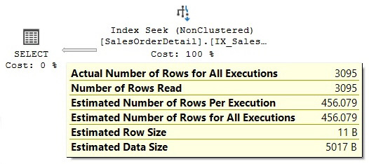
Figure 6.2 – Cardinality estimation example using a local variable
Because the Query Optimizer does not know the value of @ProductID at optimization time, the value 921 in the previous listing does not matter; any other value will give the same estimated number of rows and execution plan since it is the average number of rows per value. Finally, run this query with an inequality operator:
DECLARE @pid int = 897
SELECT * FROM Sales.SalesOrderDetail
WHERE ProductID < @pid
As mentioned previously, the value 897 does not matter; any other value will give you the same estimated number of rows and execution plan. However, this time, the Query Optimizer can’t use the density information and instead uses the standard guess of 30% selectivity for inequality comparisons. This means that the estimated number of rows is always 30% of the total number of records for an inequality operator; in this case, 30% of 121,317 is 36,395.1, as shown here:
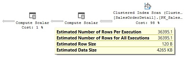
Figure 6.3 – Cardinality estimation example using a 30% guess
However, the use of local variables in a query limits the quality of the cardinality estimate when using the density information with equality operators. Worse, local variables result in no estimate at all when used with an inequality operator, which results in a guessed percentage. For this reason, local variables should be avoided in queries, and parameters or literals should be used instead. When parameters or literals are used, the Query Optimizer can use the histogram, which will provide better-quality estimates than the density information on its own.
As it happens, the last section of the DBCC SHOW_STATISTICS output is the histogram, which we will learn about in the next section.
Histograms
In SQL Server, histograms are only created for the first column of a statistics object, and they compress the information of the distribution of values in that column by partitioning that information into subsets called buckets or steps. The maximum number of steps in a histogram is 200, but even if the input contains 200 or more unique values, a histogram may still have fewer than 200 steps. To build the histogram, SQL Server finds the unique values in the column and tries to capture the most frequent ones using a variation of the maxdiff algorithm, so that the most statistically significant information is preserved. Maxdiff is one of the available histograms whose purpose is to accurately represent the distribution of data values in relational databases.
Note
You can find a simplified version of the algorithm that was used to build the histogram in the Microsoft white paper Statistics Used by the Query Optimizer in Microsoft SQL Server 2008, by Eric Hanson and Yavor Angelov.
To see how the histogram is used, run the following statement to display the current statistics of the IX_SalesOrderDetail_ProductID index on the Sales.SalesOrderDetail table:
DBCC SHOW_STATISTICS ('Sales.SalesOrderDetail', IX_SalesOrderDetail_ProductID)Both the multicolumn index and statistics objects include the ProductID, SalesOrderID, and SalesOrderDetailID columns, but because the histogram is only for the first column, this data is only available for the ProductID column.
Next, we will see some examples of how the histogram may be used to estimate the cardinality of some simple predicates. Let’s look at a section of the histogram, as shown in the following output:

RANGE_HI_KEY is the upper boundary of a histogram step; the value 826 is the upper boundary for the first step shown, while 831 is the upper boundary for the second step shown. This means that the second step may only contain values from 827 to 831. The RANGE_HI_KEY values are usually the more frequent values in the distribution.
With that in mind, and to understand the rest of the histogram structure and how the histogram information was aggregated, run the following query to obtain the real number of records for ProductIDs 827 to 831. We’ll compare them against the histogram:
SELECT ProductID, COUNT(*) AS Total
FROM Sales.SalesOrderDetail
WHERE ProductID BETWEEN 827 AND 831
GROUP BY ProductID
This produces the following output:

Going back to the histogram, EQ_ROWS is the estimated number of rows whose column value equals RANGE_HI_KEY. So, in our example, for the RANGE_HI_KEY value of 831, EQ_ROWS shows 198, which we know is also the actual number of existing records for ProductID 831.
RANGE_ROWS is the estimated number of rows whose column value falls inside the range of the step, excluding the upper boundary. In our example, this is the number of records with values from 827 to 830 (831, the upper boundary or RANGE_HI_KEY, is excluded). The histogram shows 110 records, and we could obtain the same value by getting the sum of 31 records for ProductID 827, 46 records for ProductID 828, 0 records for ProductID 829, and 33 records for ProductID 830.
DISTINCT_RANGE_ROWS is the estimated number of rows with a distinct column value inside this range, once again excluding the upper boundary. In our example, we have records for three distinct values (827, 828, and 830), so DISTINCT_RANGE_ROWS is 3. There are no records for ProductIDs 829 and 831, which is the upper boundary, which is again excluded.
Finally, AVG_RANGE_ROWS is the average number of rows per distinct value, excluding the upper boundary, and it is simply calculated as RANGE_ROWS / DISTINCT_RANGE_ROWS. In our example, we have a total of 110 records for 3 DISTINCT_RANGE_ROWS, which gives us 110 / 3 = 36.6667, also shown in the second step of the histogram shown previously. The histogram assumes the value 110 is evenly split between all three ProductIDs.
Now let’s see how the histogram is used to estimate the selectivity of some queries. Let’s look at the first query:
SELECT * FROM Sales.SalesOrderDetail
WHERE ProductID = 831
Because 831 is RANGE_HI_KEY on the second step of the histogram shown previously, the Query Optimizer will use the EQ_ROWS value (the estimated number of rows whose column value equals RANGE_HI_KEY) directly, and the estimated number of rows will be 198, as shown here:
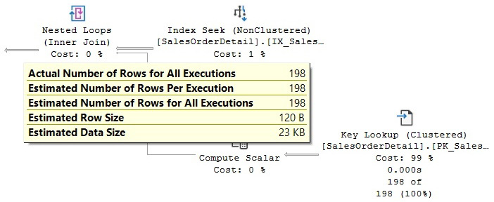
Figure 6.4 – Cardinality estimation example using a RANGE_HI_KEY value
Now, run the same query with the value set to 828. This time, the value is inside the range of the second step but is not a RANGE_HI_KEY value inside the histogram, so the Query Optimizer uses the value calculated for AVG_RANGE_ROWS (the average number of rows per distinct value), which is 36.6667, as shown in the histogram. The plan for this query is shown in Figure 6.5 and, unsurprisingly, we get the same estimated number of rows for any of the other values within the range (except for RANGE_HI_KEY). This even includes the value 829, for which there are no rows inside the table:

Figure 6.5 – Cardinality estimation example using an AVG_RANGE_ROWS value
Now, let’s use an inequality operator and try to find the records with a ProductID less than 714. Because this requires all the records, both inside the range of a step and the upper boundary, we need to calculate the sum of the values of both the RANGE_ROWS and EQ_ROWS columns for steps 1 through 7, as shown in the following histogram, which gives us a total of 13,223 rows:

The following is the query in question:
SELECT * FROM Sales.SalesOrderDetail
WHERE ProductID < 714
The estimated number of rows can be seen in the following execution plan:

Figure 6.6 – Cardinality estimation example using an inequality operator
Histograms are also used for cardinality estimations on multiple predicates; however, as of SQL Server 2022, this estimation depends on the version of the cardinality estimation used. We will cover this in the next section.
A new cardinality estimator
As mentioned in the introduction, SQL Server 2014 introduced a new cardinality estimator, and in this and later versions, the old cardinality estimator is still available. This section explains what a cardinality estimator is, why a new cardinality estimator was built, and how to enable the new and the old cardinality estimators.
The cardinality estimator is the component of the query processor whose job is to estimate the number of rows returned by relational operations in a query. This information, along with some other data, is used by the Query Optimizer to select an efficient execution plan. Cardinality estimation is inherently inexact because it is a mathematical model that relies on statistical information. It is also based on several assumptions that, although not documented, have been known over the years – some of them include the uniformity, independence, containment, and inclusion assumptions. The following is a brief description of these assumptions:
- Uniformity: This is used when the distribution for an attribute is unknown – for example, inside range rows in a histogram step or when a histogram is not available.
- Independence: This is used when the attributes in a relationship are independent unless a correlation between them is known.
- Containment: This is used when two attributes might be the same; in this case, they are assumed to be the same.
- Inclusion: This is used when comparing an attribute with a constant; it is assumed there is always a match.
The current cardinality estimator was written along with the entire query processor for SQL Server 7.0, which was released back in December 1998. This component has faced multiple changes over several years and multiple releases of SQL Server, including fixes, adjustments, and extensions to accommodate cardinality estimation for new T-SQL features. So, you may be thinking, why replace a component that has been successfully used for about the last 15 years?
In the paper Testing Cardinality Estimation Models in SQL Server, by Campbell Fraser et al., the authors explain some of the reasons for the cardinality estimator being redesigned, including the following:
- To accommodate the cardinality estimator to new workload patterns.
- Changes made to the cardinality estimator over the years made the component difficult to debug, predict, and understand.
- Trying to improve on the current model was difficult using the current architecture, so a new design was created that focused on the separation of tasks of (a) deciding how to compute a particular estimate and (b) performing the computation.
It is surprising to read in the paper that the authors admit that, according to their experience in practice, the previously listed assumptions are frequently incorrect.
A major concern that comes to mind with such a huge change inside the Query Optimizer is plan regressions. The fear of plan regressions has been considered the biggest obstacle to Query Optimizer improvements. Regressions are problems that are introduced after a fix has been applied to the Query Optimizer and are sometimes referred to as the classic two wrongs make a right. This can happen when two bad estimations – for example, the first overestimating a value and the second underestimating it – cancel each other out, luckily giving a good estimate. Correcting only one of these values may now lead to a bad estimation, which may negatively impact the choice of plan selection, thus causing a regression.
To help avoid regressions related to the new cardinality estimator, SQL Server provides a way to enable or disable it, depending on the database’s compatibility level. This can be changed using the ALTER DATABASE statement, as indicated earlier. Setting a database to compatibility level 120 will use the new cardinality estimator, whereas a compatibility level less than 120 will use the old cardinality estimator. In addition, once you are using a specific cardinality estimator, there are two trace flags you can use to change to the other. Trace flag 2312 can be used to enable the new cardinality estimator, whereas trace flag 9481 can be used to disable it. You can even use the trace flags for a specific query by using the QUERYTRACEON hint. Both trace flags and their use with the QUERYTRACEON hint are documented and supported.
Note
The compatibility level of a database will be changed several times in this chapter for demonstration purposes to show the behaviors of the old and new cardinality estimators. In a production environment, a database compatibility level should be static and never or rarely changed.
Finally, SQL Server includes several new extended events we can use to troubleshoot problems with cardinality estimation, or just to explore how it works. These events include query_optimizer_estimate_cardinality, inaccurate_cardinality_estimate, query_optimizer_force_both_cardinality_estimation_behaviors, and query_rpc_set_cardinality.
The remainder of this section will show the difference in estimations between the new and old cardinality estimators regarding AND’ed and OR’ed predicates, known as conjunctions and disjunctions, respectively. Some other sections in the chapter explain the difference in other topics (for example, when using statistics on ascending keys).
First, let’s look at the traditional behavior. For that, make sure you are using the old cardinality estimator by running the following statement on the AdventureWorks2019 database:
ALTER DATABASE AdventureWorks2019 SET COMPATIBILITY_LEVEL = 110
Then, run the following statement:
SELECT * FROM Person.Address WHERE City = 'Burbank'
By looking at the execution plan, you will see an estimate of 196 records. Similarly, the following statement will get an estimate of 194:
SELECT * FROM Person.Address WHERE PostalCode = '91502'
Both estimations of single predicates use the histogram, as explained earlier. Now, let’s use both predicates, as in the following query, which will have an estimated 1.93862 rows:
SELECT * FROM Person.Address
WHERE City = 'Burbank' AND PostalCode = '91502'
Because SQL Server doesn’t know anything about any data correlation between both predicates, it assumes they are independent and, again, uses the histograms, as we saw previously, to find the intersection between both sets of records, multiplying the selectivity of both clauses. The selectivity of the City = 'Burbank' predicate is calculated as 196 / 19,614 (where 19,614 is the total number of rows in the table), or 0.009992862. The selectivity of the PostalCode = '91502' predicate is calculated as 194 / 19,614, or 0.009890894. To get the intersection of these sets, we need to multiply the selectivity values of both predicate clauses, 0.009992862 and 0.009890894, to get 9.88383E-05. Finally, the calculated selectivity is multiplied by the total number of records to obtain the estimate, 9.88383E-05 * 19614, obtaining 1.93862. A more direct formula could be to simply use (196 * 194) / 19614.0 to get the same result.
Let’s see the same estimations while using the new cardinality estimator. To achieve this, you can use a database compatibility level newer than SQL Server 2012, which can be 120, 130, 140, 150, or 160:
ALTER DATABASE AdventureWorks2019 SET COMPATIBILITY_LEVEL = 160
GO
SELECT * FROM Person.Address WHERE City = 'Burbank' AND PostalCode = '91502'
Note
As suggested earlier, SQL Server 2022 CTP 2.0 and all SQL Server supported versions allow you to change a database to any compatibility level starting with 100, which corresponds to the SQL Server 2008 release. Trying a different value will get you error message 15048, which states Valid values of the database compatibility level are 100, 110, 120, 130, 140, 150, or 160.
Running the same statement again will give an estimate of 19.3931 rows, as shown in the following screenshot. You may need to clear the plan cache or force a new optimization if you are still getting the previous estimation:

Figure 6.7 – AND’ed predicates with the new cardinality estimator
The new formula that’s used in this case is as follows:
selectivity of most selective filter * SQRT(selectivity of next most selective filter)
This is the equivalent of (194/19614) * SQRT(196/19614) * 19614, which gives 19.393. If there were a third (or more) predicate, the formula would be extended by adding an SQRT operation for each predicate, such as in the following formula:
selectivity of most selective filter * SQRT(selectivity of next most selective filter) * SQRT(SQRT(selectivity of next most selective filter))
Now, keep in mind that the old cardinality estimator is using the original independence assumption. The new cardinality estimator is using a new formula, relaxing this assumption, which is now called the exponential backoff. This new formula does not assume total correlation either, but at least the new estimation is better than the original. Finally, note that the Query Optimizer is unable to know if the data is correlated, so it will be using these formulas, regardless of whether or not the data is correlated. In our example, the data is correlated; ZIP code 91502 corresponds to the city of Burbank, California.
Now, let’s test the same example using OR’ed predicates, first using the old cardinality estimator:
ALTER DATABASE AdventureWorks2019 SET COMPATIBILITY_LEVEL = 110
GO
SELECT * FROM Person.Address WHERE City = 'Burbank' OR PostalCode = '91502'
By definition, an OR’ed predicate is the union of the sets of rows of both clauses, without duplicates. That is, this should be the rows estimated for the City = 'Burbank' predicate, plus the rows estimated for PostalCode = '91502', but if there are any rows that may belong to both sets, then they should only be included once. As indicated in the previous example, the estimated number of rows for the City = 'Burbank' predicate alone is 196 rows, and the estimated number of rows for the PostalCode = '91502' predicate alone is 194 rows. As we saw previously, the estimated number of records that belong to both sets in the AND’ed predicate is 1.93862 rows. Therefore, the estimated number of rows for the OR’ed predicate is 196 + 194 – 1.93862, or 388.061.
Testing the same example for the new cardinality estimator would return an estimate of 292.269 rows, as shown in the following screenshot. Once again, you may need to clear the plan cache or force a new optimization if you are still getting the previous estimation:

Figure 6.8 – OR’ed predicates with the new cardinality estimator
Try the following code to see such plans:
ALTER DATABASE AdventureWorks2019 SET COMPATIBILITY_LEVEL = 160
GO
SELECT * FROM Person.Address WHERE City = 'Burbank' OR PostalCode = '91502'
The formula to obtain this estimation was suggested in the white paper Optimizing Your Query Plans with the SQL Server 2014 Cardinality Estimator, which indicates that SQL Server calculates this value by first transforming disjunctions into a negation of conjunctions. In this case, we can update our previous formula to (1-(1-(196/19614)) * SQRT(1-(194/19614))) * 19614, which returns 292.269.
If you have enabled the new cardinality estimator at the database level but want to disable it for a specific query to avoid a plan regression, you can use trace flag 9481, as explained earlier:
ALTER DATABASE AdventureWorks2019 SET COMPATIBILITY_LEVEL = 160
GO
SELECT * FROM Person.Address WHERE City = 'Burbank' AND PostalCode = '91502'
OPTION (QUERYTRACEON 9481)
Note
As indicated in Chapter 1, An Introduction to Query Optimization, the QUERYTRACEON query hint is used to apply a trace flag at the query level, and currently, it is only supported in a limited number of scenarios, including trace flags 2312 and 9481, which were mentioned in this section.
Finally, starting with SQL Server 2014, two cardinality estimators are available, so we must figure out which one was used by a specific optimization, especially for troubleshooting purposes. You can find this information on execution plans by looking at the CardinalityEstimationModelVersion property of a graphical plan or the CardinalityEstimationModelVersion attribute of the StmtSimple element in an XML plan, as shown in the following XML fragment:
<StmtSimple … CardinalityEstimationModelVersion="160" …>
A value of 70 means that the old cardinality estimator is being used. A CardinalityEstimationModelVersion value of 120 or greater means that the new cardinality estimator is being used and will match the database compatibility level.
Trace flag 4137
Finally, trace flag 4137 can be used as another choice to help with correlated AND predicates. Trace flag 4137 (which was originally released as a fix for SQL Server 2008 Service Pack 2, SQL Server 2008 R2 Service Pack 1, and SQL Server 2012 RTM) will select the lowest cardinality estimation of a list of AND’ed predicates. For example, the following code will show an estimated number of rows of 194, because 194 is the smallest of both cardinality estimations for the City = 'Burbank' and PostalCode = '91502' predicates, as explained earlier:
ALTER DATABASE AdventureWorks2019 SET COMPATIBILITY_LEVEL = 110
GO
SELECT * FROM Person.Address
WHERE City = 'Burbank' AND PostalCode = '91502'
OPTION (QUERYTRACEON 4137)
Note
Using trace flag 4137 with QUERYTRACEON is documented and supported.
To make things a little bit more confusing, trace flag 4137 does not work with the new cardinality estimator, so trace flag 9471 needs to be used instead. Another difference with trace flag 9471 is that it impacts both conjunctive and disjunctive predicates, whereas trace flag 4137 only works with conjunctive predicates.
In addition, filtered statistics, which will be covered later in this chapter, may be helpful in some cases when data is correlated.
Finally, cardinality estimation feedback, a new feature with SQL Server 2022, was designed to find if an estimation model assumption is producing a suboptimal plan and instead try a different model assumption that fits a given query and data distribution better. Cardinality estimation feedback is based on the query store and covered in more detail in Chapter 10, Intelligent Query Processing.
Cardinality estimation errors
Cardinality estimation errors can lead to the Query Optimizer making poor choices as to how best to execute a query and, therefore, to badly performing execution plans. Fortunately, you can easily check whether you have cardinality estimation errors by comparing the estimated against the actual number of rows, as shown in graphical or XML execution plans, or by using the SET STATISTICS PROFILE statement. In the following query, we will show you how to use the SET STATISTICS PROFILE statement with one of our previous examples, where SQL Server is making a blind guess regarding the selectivity of certain columns:
SET STATISTICS PROFILE ON
GO
SELECT * FROM Sales.SalesOrderDetail
WHERE OrderQty * UnitPrice > 10000
GO
SET STATISTICS PROFILE OFF
GO
This is the resulting output, with the EstimateRows column manually moved just after the Rows column, and edited to fit the page:
Rows EstimateRows StmtText

Using this output, you can easily compare the actual number of rows, shown on the Rows column, against the estimated number of records, shown on the EstimateRows column, for each operator in the plan. Introduced with SQL Server 2012, the inaccurate_cardinality_estimate extended event can also be used to detect inaccurate cardinality estimations by identifying which query operators output significantly more rows than those estimated by the Query Optimizer.
Because each operator relies on previous operations for its input, cardinality estimation errors can propagate exponentially throughout the query plan. For example, a cardinality estimation error on a Filter operator can impact the cardinality estimation of all the other operators in the plan that consume the data produced by that operator. If your query is not performing well and you find cardinality estimation errors, check for problems such as missing or out-of-date statistics, very small samples being used, correlation between columns, use of scalar expressions, guessing selectivity issues, and so on.
Recommendations to help with these issues have been provided throughout this chapter and include topics such as using the auto-create and auto-update statistics default configurations, updating statistics using WITH FULLSCAN, avoiding local variables in queries, avoiding non-constant-foldable or complex expressions on predicates, using computed columns, and considering multicolumn or filtered statistics, among other things. In addition, parameter sniffing and parameter-sensitive queries will be covered in more detail in Chapter 8, Understanding Plan Caching. That’s a fairly long list, but it should help convince you that you are already armed with pragmatically useful information.
Some SQL Server features, such as table variables, have no statistics, so you may want to consider using a temporary table or a standard table instead if you’re having performance problems related to cardinality estimation errors. Multistatement table-valued user-defined functions have no statistics either. In this case, you can consider using a temporary table or a standard table as a temporary holding place for their results. In both these cases (table variables and multistatement table-valued user-defined functions), the Query Optimizer will guess at one row (which has been updated to 100 rows for multistatement table-valued user-defined functions in SQL Server 2014). In addition, for complex queries that are not performing well because of cardinality estimation errors, you may want to consider breaking down the query into two or more steps while storing the intermediate results in temporary tables. This will allow SQL Server to create statistics on the intermediate results, which will help the Query Optimizer produce a better execution plan. More details about breaking down complex queries will be covered in Chapter 12, Understanding Query Hints.
Note
A new trace flag, 2453, was introduced with SQL Server 2012 Service Pack 2 and SQL Server 2014, which provides better cardinality estimation while using table variables. For more details, see http://support.microsoft.com/kb/2952444.
Now that we have learned about cardinality estimation, we will explore another key feature in SQL Server: incremental statistics.
Incremental statistics
A major problem with updating statistics in large tables in SQL Server was that the entire table always had to be sampled, even if only recent data had changed. This was also true when partitioning was being used: even if only the newest partition had changed since the last time statistics were updated, updating statistics again required sampling the entire table, including all the partitions that hadn’t changed. Incremental statistics, a feature introduced with SQL Server 2014, can help with this problem.
Using incremental statistics, you can only update the statistics on the partition or partitions that have been modified, and the information on these partitions will be merged with the existing information to create the final statistics object. Another advantage of incremental statistics is that the percentage of data changes required to trigger an automatic update of the statistics now works at the partition level, instead of the table level. Unfortunately, the histogram is still limited to 200 steps for the entire statistics object in this version of SQL Server.
Let’s look at an example of how to update statistics at the partition level to explore its behavior. First, we need to create a partitioned table using the AdventureWorks2019 database:
CREATE PARTITION FUNCTION TransactionRangePF1 (datetime)
AS RANGE RIGHT FOR VALUES
(
'20130901', '20131001', '20131101', '20131201',
'20140101', '20140201', '20140301', '20140401',
'20140501', '20140601', '20140701'
)
GO
CREATE PARTITION SCHEME TransactionsPS1 AS PARTITION TransactionRangePF1 TO
(
[PRIMARY], [PRIMARY], [PRIMARY], [PRIMARY], [PRIMARY],
[PRIMARY], [PRIMARY], [PRIMARY], [PRIMARY], [PRIMARY],
[PRIMARY], [PRIMARY], [PRIMARY]
)
GO
CREATE TABLE dbo.TransactionHistory
(
TransactionID int NOT NULL,
ProductID int NOT NULL,
ReferenceOrderID int NOT NULL,
ReferenceOrderLineID int NOT NULL DEFAULT (0),
TransactionDate datetime NOT NULL DEFAULT (GETDATE()),
TransactionType nchar(1) NOT NULL,
Quantity int NOT NULL,
ActualCost money NOT NULL,
ModifiedDate datetime NOT NULL DEFAULT (GETDATE()),
CONSTRAINT CK_TransactionType
CHECK (UPPER(TransactionType) IN (N'W', N'S', N'P'))
)
ON TransactionsPS1 (TransactionDate)
GO
Note
For details about partitioning and the CREATE PARTITION FUNCTION/SCHEME statements, please refer to Partitioned Tables and Indexes in the SQL Server documentation.
We currently have data to populate 12 partitions. Let’s start by populating only 11:
INSERT INTO dbo.TransactionHistory
SELECT * FROM Production.TransactionHistory
WHERE TransactionDate < '2014-07-01'
If required, you can use the following query to inspect the contents of the partitions, where you will see that all the partitions except the last one are now populated:
SELECT * FROM sys.partitions
WHERE object_id = OBJECT_ID('dbo.TransactionHistory')Let’s create an incremental statistics object using the CREATE STATISTICS statement with the new INCREMENTAL clause set to ON (OFF is the default):
CREATE STATISTICS incrstats ON dbo.TransactionHistory(TransactionDate)
WITH FULLSCAN, INCREMENTAL = ON
You can also create incremental statistics while creating an index using the new STATISTICS_INCREMENTAL clause of the CREATE INDEX statement. You can inspect the created statistics object using the following query:
DBCC SHOW_STATISTICS('dbo.TransactionHistory', incrstats)Among other things, you will notice that the created histogram has 200 steps (only the last three are shown here):

So, we already have the maximum number of steps in a statistics object. What would happen if we added data to a new partition? Let’s add data to partition 12:
INSERT INTO dbo.TransactionHistory
SELECT * FROM Production.TransactionHistory
WHERE TransactionDate >= '2014-07-01'
Now, we must update the statistics object using the following statement:
UPDATE STATISTICS dbo.TransactionHistory(incrstats)
WITH RESAMPLE ON PARTITIONS(12)
Note the new syntax specifying the partition, where you can specify multiple partitions, separated by commas. The UPDATE STATISTICS statement reads the specified partitions and then merges their results with the existing statistics object to build the global statistics. Note the RESAMPLE clause; this is required because partition statistics objects need to have the same sample rates to be merged to build the global statistics objects. Although only the specified partition was scanned, you can see that SQL Server has rearranged the histogram. The last three steps now show data for the added partition. You can also compare the original histogram with the new one for other minor differences:

If you want to disable the incremental statistics object for any reason, you can use the following statement to go back to the original behavior (or optionally just drop the statistics object and create a new one):
UPDATE STATISTICS dbo.TransactionHistory(incrstats)
WITH FULLSCAN, INCREMENTAL = OFF
After disabling the incremental statistics, trying to update a partition, as shown previously, will return the following error message:
Msg 9111, Level 16, State 1, Line 1
UPDATE STATISTICS ON PARTITIONS syntax is not supported for non-incremental statistics.
Finally, you can also enable incremental statistics for your automatic statistics at the database level, if needed. This requires the INCREMENTAL = ON clause in the ALTER DATABASE statement and also requires AUTO_CREATE_STATISTICS to be set to ON.
To clean up the objects that were created for this exercise, run the following statements:
DROP TABLE dbo.TransactionHistory
DROP PARTITION SCHEME TransactionsPS1
DROP PARTITION FUNCTION TransactionRangePF1
With this, we have learned all about incremental statistics and how to use it. In the next section, we will learn how to apply statistics to computed columns.
Statistics on computed columns
Another interesting step that’s performed during query optimization is automatically matching computed columns. Although computed columns have been available in previous versions of SQL Server, the automatic matching feature was only introduced with SQL Server 2005. In this section, we will show you how this feature works and explain how computed columns can help improve the performance of your queries.
A problem that’s faced by some queries that use scalar expressions is that they usually cannot benefit from statistics, and without statistics, the Query Optimizer will use the 30% selectivity guess on inequality comparisons, which may produce inefficient execution plans. A solution to this problem is using computed columns since SQL Server can automatically create and update statistics on these columns. A great benefit of this solution is that you do not need to specify the name of the computed column in your queries for SQL Server to use its statistics. The Query Optimizer automatically matches the computed column definition to an existing scalar expression in a query, so your applications do not need to be changed.
To see an example, run the following query:
SELECT * FROM Sales.SalesOrderDetail
WHERE OrderQty * UnitPrice > 10000
This creates the following plan:

Figure 6.9 – Cardinality estimation example using a 30% guess
The estimated number of rows is 36,395.1, which is 30% of the total number of rows (121,317), although the query returns only 772 records. SQL Server is using a selectivity guess because it cannot estimate the selectivity of the OrderQty * UnitPrice > 10000 expression.
Now, create a computed column:
ALTER TABLE Sales.SalesOrderDetail
ADD cc AS OrderQty * UnitPrice
Run the previous SELECT statement again and note that, this time, the estimated number of rows has changed and is close to the actual number of rows returned by the query, as shown in the following screenshot. Optionally, you can test replacing 10,000 with some other value, such as 10, 100, 1,000, or 5,000, and compare the actual and the estimated number of rows returned:

Figure 6.10 – Cardinality estimation example using computed columns
Note that creating the computed column does not create statistics; these statistics are created the first time the query is optimized. You can run the following query to display the information about the statistics objects for the Sales.SalesOrderDetail table:
SELECT * FROM sys.stats
WHERE object_id = OBJECT_ID('Sales.SalesOrderDetail')The newly created statistics object will most likely be at the end of the list. Copy the name of the object and use the following command to display the details about the statistics object (we have used the name of my local object here, but you should replace that as appropriate):
DBCC SHOW_STATISTICS ('Sales.SalesOrderDetail', _WA_Sys_0000000E_44CA3770)You can also use cc as the name of the object to get the same results. The cc column should be shown on the Columns field in the density section. In any case, the number of rows is estimated using the histogram of the created statistics object, as explained earlier for inequality comparisons:
DBCC SHOW_STATISTICS ('Sales.SalesOrderDetail', cc)Unfortunately, and still true for SQL Server 2022, for automatic matching to work, the expression must be the same as the computed column definition. So, if we change the query to UnitPrice * OrderQty instead of OrderQty * UnitPrice, the execution plan will show an estimated number of rows of 30% again, as shown by the following query:
SELECT * FROM Sales.SalesOrderDetail
WHERE UnitPrice * OrderQty > 10000
Finally, drop the created computed column:
ALTER TABLE Sales.SalesOrderDetail
DROP COLUMN cc
Now, let’s check out some filtered statistics.
Filtered statistics
Filtered statistics are statistics created on a subset of records in a table. Filtered statistics are automatically created when filtered indexes are created, but they can also be created manually by specifying a WHERE clause on the CREATE STATISTICS statement, in which case a filtered index is not required. As you may imagine, filtered statistics can help with queries accessing specific subsets of data. They can also be useful in situations such as correlated columns, especially when one of these columns has a small number of unique values, and you can create multiple filtered statistics for each of these distinct values. As shown in the Histogram section, when using multiple predicates, SQL Server assumes that each clause in a query is independent. If the columns used in this query were correlated, then the cardinality estimation would be incorrect. Even with the exponential backoff behavior of the new cardinality estimator, you can still get better cardinality estimation with filter statistics because each statistics object has its own histogram. Filtered statistics may also help with huge tables where a large number of unique values are not accurately represented in the 200-step limitation currently enforced on histograms.
Next, we learn how to use filtered statistics to help in a problem with correlated columns. Running the following query will correctly estimate the number of rows to be 93:
SELECT * FROM Person.Address
WHERE City = 'Los Angeles'
In the same way, running the following query will correctly estimate 4,564 rows:
SELECT * FROM Person.Address
WHERE StateProvinceID = 9
However, because StateProvinceID 9 corresponds to the state of California (which you can verify by looking at the Person.StateProvince table), somebody can run this query, which in this case will show a less precise estimate of 44.8614 rows (this is using the new cardinality estimator, or 21.6403 using the old one):
SELECT * FROM Person.Address
WHERE City = 'Los Angeles' AND StateProvinceID = 9
This can be seen in the following plan:

Figure 6.11 – Cardinality estimate with exponential backoff
Because of the assumption of independence, SQL Server will multiply the cardinality of both predicates, as explained earlier in this chapter. The calculation, abbreviated as (93 * 4,564) / 19,614, will give us a value of 21.6403 for the old cardinality estimator (19,614 is the total number of rows in the table). In the case of the exponential backoff used by the new cardinality estimator, the calculation would be (93 / 19,614) * SQRT(4,564 / 19,614) * 19,614, which will be roughly 44.861 rows.
However, both the independence assumption and the exponential backoff are incorrect in this example because the columns are statistically correlated. To help with this problem, you can create a filtered statistics object for the state of California, as shown in the following statement:
CREATE STATISTICS california
ON Person.Address(City)
WHERE StateProvinceID = 9
Clearing the cache and running the previous query again will now give a better estimate:
DBCC FREEPROCCACHE
GO
SELECT * FROM Person.Address
WHERE City = 'Los Angeles' AND StateProvinceID = 9
This can be seen in the following plan:

Figure 6.12 – Cardinality estimate with filtered statistics
Now, let’s inspect the filtered statistics object by running the following statement:
DBCC SHOW_STATISTICS('Person.Address', california)This will produce the following output (edited here to fit the page), showing the estimate of 93 rows for Los Angeles on the EQ_ROWS column:

Notice that the filter definition is shown on the Filter Expression field and that the Unfiltered Rows field shows the total number of records in the table when the filtered statistics were created. Also, note that this time, the Rows column number is less than the total number of rows in the table and corresponds to the number of records that satisfied the filter predicate when the statistics object was created. The filter definition can also be seen on the filter_definition column of the sys.stats catalog view. Also, notice that the histogram only shows cities for California, according to the filter definition (only a few steps are shown).
Finally, drop the statistics object you have just created by running the following statement:
DROP STATISTICS Person.Address.california
Now, let’s explore more functions for statistics.
Statistics on ascending keys
Statistics on ascending keys presents a cardinality estimation problem that has been present in all versions of SQL Server since version 7. Using trace flags 2389 and 2390 has been the best solution to this problem. Starting with SQL Server 2014, you can also use the new cardinality estimator to obtain the same estimation, but without having to use these trace flags.
But first, let’s explain what the problem is. As we saw earlier, SQL Server builds a histogram on the first column of each statistics object. With statistics on ascending or descending key columns, such as IDENTITY and real-time timestamp columns, newly inserted values usually fall outside the range of values covered by the histogram. In addition, the number of records added might be too small to trigger an automatic update of statistics. Because recently added rows are not covered in the histogram when a significant number of rows should be included, running a query using those values may result in inaccurate cardinality estimates, which may also result in poorly performing plans.
The traditional recommendation from Microsoft to fix this problem has been to manually update statistics after loading data, but unfortunately, this may also require more frequent statistics updates, which may not always be feasible. Trace flags 2389 and 2390, which were first published by Ian Jose from Microsoft in his article Ascending Keys and Auto Quick Corrected Statistics, were also introduced with SQL Server 2005 Service Pack 1 to help with this problem.
To show you what the problem is and how these trace flags work, let’s start by creating a table in AdventureWorks2019. But first, make sure you are using the old cardinality estimator:
ALTER DATABASE AdventureWorks2019 SET COMPATIBILITY_LEVEL = 110
GO
CREATE TABLE dbo.SalesOrderHeader (
SalesOrderID int NOT NULL,
RevisionNumber tinyint NOT NULL,
OrderDate datetime NOT NULL,
DueDate datetime NOT NULL,
ShipDate datetime NULL,
Status tinyint NOT NULL,
OnlineOrderFlag dbo.Flag NOT NULL,
SalesOrderNumber nvarchar(25) NOT NULL,
PurchaseOrderNumber dbo.OrderNumber NULL,
AccountNumber dbo.AccountNumber NULL,
CustomerID int NOT NULL,
SalesPersonID int NULL,
TerritoryID int NULL,
BillToAddressID int NOT NULL,
ShipToAddressID int NOT NULL,
ShipMethodID int NOT NULL,
CreditCardID int NULL,
CreditCardApprovalCode varchar(15) NULL,
CurrencyRateID int NULL,
SubTotal money NOT NULL,
TaxAmt money NOT NULL,
Freight money NOT NULL,
TotalDue money NOT NULL,
Comment nvarchar(128) NULL,
rowguid uniqueidentifier NOT NULL,
ModifiedDate datetime NOT NULL
)
Populate the table with some initial data and create an index on it (notice that both tables have the same name, but in the dbo and Sales schemas, respectively):
INSERT INTO dbo.SalesOrderHeader SELECT * FROM Sales.SalesOrderHeader
WHERE OrderDate < '2014-06-19 00:00:00.000'
CREATE INDEX IX_OrderDate ON SalesOrderHeader(OrderDate)
After creating the index, SQL Server will also create a statistics object for it, so a query like this will have a good cardinality estimate of 35 rows (as there is data for July 19, and it is captured on the last step of the statistics histogram object, which you can verify by using the DBCC SHOW_STATISTICS statement):
SELECT * FROM dbo.SalesOrderHeader WHERE OrderDate = '2014-06-18 00:00:00.000'
Now, let’s suppose we add new data for June 19:
INSERT INTO dbo.SalesOrderHeader SELECT * FROM Sales.SalesOrderHeader
WHERE OrderDate = '2014-06-19 00:00:00.000'
So, let’s change the query to look for records for June 19:
SELECT * FROM dbo.SalesOrderHeader WHERE OrderDate = '2014-06-19 00:00:00.000'
Because the number of rows added is not enough to trigger an automatic update of statistics, June 19 is not represented on the existing histogram. This anomaly means that SQL Server will use an estimate of 1, as shown here:

Figure 6.13 – Bad cardinality estimate after new records are added
Although the plans for both queries in this example are very similar, a bad cardinality estimate may produce bad plans in some more realistic scenarios and queries.
Trace flag 2389
Now, let’s see how trace flag 2389 helps with this problem. Run the following statements (notice that trace flag 2388 has not been mentioned before and will be explained shortly):
DBCC TRACEON (2388)
DBCC TRACEON (2389)
Trace flag 2389, which was introduced with SQL Server 2005 Service Pack 1, begins to track the nature of columns via subsequent operations of updating statistics. When the statistics are seen to increase three times in a row, the column is branded Ascending. Trace flag 2388 is not required to enable the behavior described in this article but enables previously hidden metadata to be displayed. This is useful to show how trace flags 2389 and 2390 work and determine if a column has been branded as Ascending. The trace flag changes the output of the DBCC SHOW_STATISTICS statement to show you a historical view of the most recent statistics update operations.
Trace flag 2390 enables a similar behavior to 2389, even if the ascending nature of the column is not known, but we will not cover that here. Run DBCC SHOW_STATISTICS:
DBCC SHOW_STATISTICS ('dbo.SalesOrderHeader', 'IX_OrderDate')The statement shows the following output (condensed to fit the page):

There’s not much data for now. However, we will show you this output after three consecutive batches of inserting data and updating statistics. Run the following statement to update the statistics, including the data you just added for June 19:
UPDATE STATISTICS dbo.SalesOrderHeader WITH FULLSCAN
DBCC SHOW_STATISTICS now shows the following:

Here, Rows Above and Inserts Since Last Update account for the 30 rows that were added previously (you may need to scroll to the right). Now, run the second batch for June 20:
INSERT INTO dbo.SalesOrderHeader SELECT * FROM Sales.SalesOrderHeader
WHERE OrderDate = '2014-06-20 00:00:00.000'
Again, running this query will verify the one-row estimate in the plan:
SELECT * FROM dbo.SalesOrderHeader WHERE OrderDate = '2014-06-20 00:00:00.000'
Now, update the statistics again:
UPDATE STATISTICS dbo.SalesOrderHeader WITH FULLSCAN
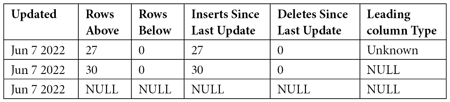
DBCC SHOW_STATISTICS now shows the following. Notice a new record with Inserts Since Last Update and Rows Above, with a value of 27. Leading column Type still shows Unknown:
Now, it’s time for a third batch:
INSERT INTO dbo.SalesOrderHeader SELECT * FROM Sales.SalesOrderHeader
WHERE OrderDate = '2014-06-21 00:00:00.000'
Update the statistics one last time:
UPDATE STATISTICS dbo.SalesOrderHeader WITH FULLSCAN
DBCC SHOW_STATISTICS now shows this:

In addition to the new record accounting for the 32 rows that were added, you will notice that the branding was changed to Ascending. Once the column is branded as Ascending, SQL Server will be able to give you a better cardinality estimate, without having to manually update the statistics. To test it, try this batch:
INSERT INTO dbo.SalesOrderHeader SELECT * FROM Sales.SalesOrderHeader
WHERE OrderDate = '2014-06-22 00:00:00.000'
Now, run the following query:
SELECT * FROM dbo.SalesOrderHeader WHERE OrderDate = '2014-06-22 00:00:00.000'
This time, we get a better cardinality estimate. Notice that UPDATE STATISTICS wasn’t required this time. Instead of the estimate of one row, now, we get 27.9677. But where is this value coming from? The Query Optimizer is now using the density information of the statistics object. As explained earlier, the definition of density is 1 / "number of distinct values," and the estimated number of rows is obtained using the density multiplied by the number of records in the table, which in this case is 0.000896861 * 31184, or 27.967713424, as shown in the plan. Also, notice that density information is only used for values not covered in the histogram (you can see the density information using the same DBCC SHOW_STATISTICS statement, but in another session where trace flag 2388 is not enabled).
In addition, if we look for data that does not exist, we still get the one-row estimate, which is always adequate because it will return 0 records:
SELECT * FROM dbo.SalesOrderHeader WHERE OrderDate = '2014-06-23 00:00:00.000'
Notice that branding a column as Ascending requires statistics to increase three times in a row. If we insert older data later, breaking the ascending sequence, the Leading column Type column will show as Stationary and the query processor will be back to the original cardinality estimate behavior. Making three new additional updates to a row with increasing values can brand it as Ascending again.
Finally, you could use the trace flags on a query without defining them at the session or global level using the QUERYTRACEON hint, as shown here:
SELECT * FROM dbo.SalesOrderHeader WHERE OrderDate = '2014-06-22 00:00:00.000'
OPTION (QUERYTRACEON 2389, QUERYTRACEON 2390)
Trace flags 2389 and 2390 are no longer needed if you are using the new cardinality estimator, and you will get the same behavior and estimation. To see how it works, drop the dbo.SalesOrderHeader table:
DROP TABLE dbo.SalesOrderHeader
Disable trace flags 2388 and 2389, as shown here, or open a new session:
DBCC TRACEOFF (2388)
DBCC TRACEOFF (2389)
Note
You can also make sure that the trace flags are not enabled by running DBCC TRACESTATUS.
Create dbo.SalesOrderHeader, as indicated at the beginning of this section. Insert some data again and create an index, as shown here:
INSERT INTO dbo.SalesOrderHeader SELECT * FROM Sales.SalesOrderHeader
WHERE OrderDate < '2014-06-19 00:00:00.000'
CREATE INDEX IX_OrderDate ON SalesOrderHeader(OrderDate)
Now, add new data for June 19:
INSERT INTO dbo.SalesOrderHeader SELECT * FROM Sales.SalesOrderHeader
WHERE OrderDate = '2014-06-19 00:00:00.000'
This is the same as we got previously because the number of rows that we’ve added is too small – it is not enough to trigger an automatic update of statistics. Running the following query with the old cardinality estimator will estimate one row, as we saw earlier:
ALTER DATABASE AdventureWorks2019 SET COMPATIBILITY_LEVEL = 110
GO
SELECT * FROM dbo.SalesOrderHeader WHERE OrderDate = '2014-06-19 00:00:00.000'
Running the same query with the new cardinality estimator will give a better estimate of 27.9631, without the need to use trace flags 2390 and 2390:
ALTER DATABASE AdventureWorks2019 SET COMPATIBILITY_LEVEL = 160
GO
SELECT * FROM dbo.SalesOrderHeader WHERE OrderDate = '2014-06-19 00:00:00.000'
27.9631 is estimated the same way as explained earlier – that is, using the density multiplied by the number of records in the table, which in this case is 0.0008992806 * 31095, or 27.9631302570. But remember to use DBCC SHOW_STATISTICS against this new version of the table to obtain the new density.
Now that we have covered various statistics functions, we will explore some unique options that are part of the UPDATE STATISTICS statement.
UPDATE STATISTICS with ROWCOUNT and PAGECOUNT
The undocumented ROWCOUNT and PAGECOUNT options of the UPDATE STATISTICS statement are used by the Data Engine Tuning Advisor (DTA) to script and copy statistics when you want to configure a test server to tune the workload of a production server. You can also see these statements in action if you script a statistics object. As an example, try the following in Management Studio: select Databases, right-click the AdventureWorks2019 database, select Tasks, Generate Scripts…, click Next, select Select specific database objects, expand Tables, select Sales.SalesOrderDetail, click Next, click Advanced, look for the Script Statistics choice, and select Script statistics and histograms. Finally, choose True for Script Indexes. Click OK and finish the wizard to generate the scripts. You will get a script with a few UPDATE STATISTICS statements, similar to what’s shown here (with the STATS_STREAM value shortened to fit this page):
UPDATE STATISTICS [Sales].[SalesOrderDetail]([IX_SalesOrderDetail_ProductID])
WITH STATS_STREAM = 0x010000000300000000000000 …, ROWCOUNT = 121317,
PAGECOUNT = 274
In this section, you will learn how to use the ROWCOUNT and PAGECOUNT options of the UPDATE STATISTICS statement in cases where you want to see which execution plans would be generated for huge tables (for example, with millions of records), but then test those plans in small or even empty tables. As you can imagine, these options can be helpful for testing in some scenarios where you may not want to spend time or disk space creating big tables.
By using this method, you are asking the Query Optimizer to generate execution plans using cardinality estimations as if the table contained millions of records, even if your table is tiny or empty. Note that this option, available since SQL Server 2005, only helps in creating the execution plan for your queries. Running the query will use the real data in your test table, which will, of course, execute faster than a table with millions of records.
Using these UPDATE STATISTICS options does not change the table statistics – it only changes the counters for the numbers of rows and pages of a table. As we will see shortly, the Query Optimizer uses this information to estimate the cardinality of queries. Finally, before we look at examples, keep in mind that these are undocumented and unsupported options and should not be used in a production environment.
So, let’s look at an example. Run the following query to create a new table on the Adventure Works2019 database:
SELECT * INTO dbo.Address
FROM Person.Address
Inspect the number of rows by running the following query; the row_count column should show 19,614 rows:
SELECT * FROM sys.dm_db_partition_stats
WHERE object_id = OBJECT_ID('dbo.Address')Now, run the following query and inspect the graphical execution plan:
SELECT * FROM dbo.Address
WHERE City = 'London'
Running this query will create a new statistics object for the City column and will show the following plan. Note that the estimated number of rows is 434 and that it’s using a simple Table Scan operator:

Figure 6.14 – Cardinality estimation example using a small table
We can discover where the Query Optimizer is getting the estimated number of rows by inspecting the statistics object. Using the methodology shown in the Histogram section, you can find out the name of the statistics object and then use DBCC SHOW_STATISTICS to show its histogram. By looking at the histogram, you can find a value of 434 on EQ_ROWS for the RANGE_HI_KEY value 'London'.
Now, run the following UPDATE STATISTICS WITH ROWCOUNT, PAGECOUNT statement (you can specify any other value for ROWCOUNT and PAGECOUNT):
UPDATE STATISTICS dbo.Address WITH ROWCOUNT = 1000000, PAGECOUNT = 100000
If you inspect the number of rows from sys.dm_db_partition_stats again, as shown previously, it will now show 1,000,000 rows (the new number of pages is also shown by the in_row_data_page_count column). Clear the plan cache and run the query again:
DBCC FREEPROCCACHE
GO
SELECT * FROM dbo.Address WHERE City = 'London'
Note that the estimated number of rows has changed from 434 to 22,127.1, as shown here:

Figure 6.15 – Cardinality estimation using ROWCOUNT and PAGECOUNT
However, if you look at the statistics object again while using DBCC SHOW_STATISTICS, as shown previously, you’ll see that the histogram has not changed. One way to obtain the estimated number of rows shown in the new execution plan is by calculating the percentage (or fraction) of rows for London from the statistics sample, which in this case is 19,614. So, the fraction is 434 / 19,614, or 0.022127052. Next, we apply the same percentage to the new "current" number of rows, which results in 1,000,000 * 0.022127052, and we get 22,127.1, which is the estimated number of rows displayed in the preceding plan.
Finally, if you want to restore the real values for rows and pages, perhaps to perform additional testing, you can use the DBCC UPDATEUSAGE statement. DBCC UPDATEUSAGE can be used to correct pages and row count inaccuracies in the catalog views. Run the following statement:
DBCC UPDATEUSAGE(AdventureWorks2019, 'dbo.Address') WITH COUNT_ROWS
However, after you finish your testing, it is recommended that you drop this table to avoid any page and row count inaccuracies left by mistake:
DROP TABLE dbo.Address
Now that we know how to work with various statistics options, we will learn how to maintain and update them.
Statistics maintenance
As mentioned previously, the Query Optimizer will, by default, automatically update statistics when they are out of date. Statistics can also be updated with the UPDATE STATISTICS statement, which you can schedule to run as a maintenance job. Another statement that’s commonly used, sp_updatestats, also runs UPDATE STATISTICS behind the scenes.
There are two important benefits of updating statistics in a maintenance job. The first is that your queries will use updated statistics without having to wait for the statistics to be automatically updated, thus avoiding delays in the optimization of your queries (although asynchronous statistics updates can also be used to partially help with this problem). The second benefit is that you can use a bigger sample than the Query Optimizer will use, or you can even scan the entire table. This can give you better-quality statistics for big tables, especially for those where data is not randomly distributed in their data pages. Manually updating statistics can also be a benefit after operations such as batch data loads, which update large amounts of data, are performed.
On the other hand, note that updating the statistics will cause plans already in the plan cache that are using these statistics to be compiled, so you may not want to update statistics too frequently either.
An additional consideration for manually updating statistics in a maintenance job is how they relate to index rebuild maintenance jobs, which also update the index statistics. Keep the following items in mind when combining maintenance jobs for both indexes and statistics, remembering that there are both index and non-index column statistics, and that index operations may only impact the first of these:
- Rebuilding an index (for example, by using the ALTER INDEX … REBUILD statement) will also update index statistics by scanning all the rows in the table, which is the equivalent of using UPDATE STATISTICS WITH FULLSCAN. Rebuilding indexes does not update any column statistics.
- Reorganizing an index (for example, using the ALTER INDEX … REORGANIZE statement) does not update any statistics, not even index statistics.
- By default, the UPDATE STATISTICS statement updates both index and column statistics. Using the INDEX option will only update index statistics while using the COLUMNS option will only update nonindexed column statistics.
Therefore, depending on your maintenance jobs and scripts, several scenarios can exist. The simplest maintenance plan is if you want to rebuild all the indexes and update all the statistics. As mentioned previously, if you rebuild all your indexes, then all the index statistics will also be automatically updated by scanning all the rows in the table. Then, you just need to update your non-indexed column statistics by running UPDATE STATISTICS WITH FULLSCAN, COLUMNS. Because the index rebuild job only updates index statistics, and the second one only updates column statistics, it does not matter which one is executed first.
Of course, more complicated maintenance plans exist – for example, when indexes are rebuilt or reorganized depending on their fragmentation level, a topic that was covered in more detail in Chapter 5, Working with Indexes. You should keep the items mentioned previously in mind so that you can avoid problems such as updating the index statistics twice, which could occur when both the index rebuild and update statistics operations are performed. You should also avoid discarding previously performed work – for example, when you rebuild the indexes of a table, which also updates statistics by scanning the entire table – and later running a job that updates the statistics with the default or smaller sample. In this case, previously updated statistics are replaced with statistics that have potentially less quality.
Let me show you how these commands work with some examples. Create a new table called dbo.SalesOrderDetail:
SELECT * INTO dbo.SalesOrderDetail FROM Sales.SalesOrderDetail
The following query uses the sys.stats catalog view to show that there are no statistics objects for the new table:
SELECT name, auto_created, STATS_DATE(object_id, stats_id) AS update_date
FROM sys.stats
WHERE object_id = OBJECT_ID('dbo.SalesOrderDetail')Now, run the following query:
SELECT * FROM dbo.SalesOrderDetail
WHERE SalesOrderID = 43670 AND OrderQty = 1
Use the previous query using sys.stats to verify that two statistics objects were created – one for the SalesOrderID column and a second for the OrderQty column. Now, create the following index and run the sys.stats query again to verify that a new statistics object for the ProductID column has been created:
CREATE INDEX IX_ProductID ON dbo.SalesOrderDetail(ProductID)
The following table shows the output of the sys.stats query so far:

Notice how the value of the auto_created column, which indicates whether the statistics were created by the Query Optimizer, is 0 for the IX_ProductID statistics object. Run the following command to update just the column statistics:
UPDATE STATISTICS dbo.SalesOrderDetail WITH FULLSCAN, COLUMNS
You can validate that only the column statistics were updated by comparing the update_date column with the previous output. The update_date column uses the STATS_DATE function to display the last point in time when the statistics were updated, as shown in the following output:

This command will do the same for just the index statistics:
UPDATE STATISTICS dbo.SalesOrderDetail WITH FULLSCAN, INDEX
The following commands will update both the index and column statistics:
UPDATE STATISTICS dbo.SalesOrderDetail WITH FULLSCAN
UPDATE STATISTICS dbo.SalesOrderDetail WITH FULLSCAN, ALL
As mentioned earlier, if you run the sys.stats query after each of the following two queries, you’ll see how an ALTER INDEX REBUILD statement only updates index statistics:
ALTER INDEX ix_ProductID ON dbo.SalesOrderDetail REBUILD
You can verify that reorganizing an index does not update any statistics like so:
ALTER INDEX ix_ProductID on dbo.SalesOrderDetail REORGANIZE
Finally, for good housekeeping, remove the table you have just created:
DROP TABLE dbo.SalesOrderDetail
Finally, we strongly recommend using Ola Hallengren’s SQL Server maintenance solution for SQL Server backup, integrity check, and index and statistics maintenance jobs. Ola Hallengren’s SQL Server maintenance solution is free and you can find it at https://ola.hallengren.com.
Cost estimation
As we have established, the quality of the execution plans the Query Optimizer generates is directly related to the accuracy of its costing estimates. Even when the Query Optimizer can enumerate low-cost plans, an incorrect cost estimation may result in the Query Optimizer choosing inefficient plans, which can negatively impact the performance of your database. During query optimization, the Query Optimizer explores many candidate plans, estimates their cost, and then selects the most efficient one.
Costs are estimated for any partial or complete plan, as shown in Chapter 3, The Query Optimizer, when we explored the content of the Memo structure. Cost computation is done per operator, and the total plan cost is the sum of the costs of all the operators in that plan. The cost of each operator depends on its algorithm and the estimated number of records it returns.
Some operators, such as Sort and Hash Join, also consider the available memory in the system. A high-level overview of the cost of the algorithms for some of the most used operators was provided in Chapter 4, The Execution Engine.
So, each operator has an associated CPU cost; some of them will also have some I/O cost, and the cost of the operator as a whole is the sum of these costs. An operator such as a Clustered Index Scan has both CPU and I/O costs, whereas some other operators, such as Stream Aggregate, will only have a CPU cost. Because it is not documented how these costs are calculated, I will show you a basic example of how the cost of a plan is estimated.
To demonstrate this in an example, let’s look at the largest table in the AdventureWorks database. Run the following query and look at the estimated CPU and I/O costs for the Clustered Index Scan operator:
SELECT * FROM Sales.SalesOrderDetail
WHERE LineTotal = 35
Note that in an older version of SQL Server, when the current Query Optimizer was built, the cost used to mean the estimated time in seconds that a query would take to execute on a specific hardware configuration. However, at the time of writing, this value is meaningless as an objective unit of measurement and should not be interpreted as one. Its purpose is to solely be used internally to pick between different candidate plans.
For a Clustered Index Scan operator, it has been observed that the CPU cost is 0.0001581 for the first record, plus 0.0000011 for any additional record after that. Because we have an estimated 121,317 records here, we can calculate 0.0001581 + 0.0000011 * (121317 – 1), which comes to 0.133606, which is the value shown as Estimated CPU Cost in Figure 6.17. Similarly, we noticed that the minimum I/O cost is 0.003125 for the first database page, and then it grows in increments of 0.00074074 for every additional page. Because this operator scans the entire table, we can use the following query to find the number of database pages (which turns out to be 1,239):
SELECT in_row_data_page_count, row_count
FROM sys.dm_db_partition_stats
WHERE object_id = OBJECT_ID('Sales.SalesOrderDetail')AND index_id = 1
In this case, we have 0.003125 + 0.00074074 * (1238), which comes to roughly 0.920162, which is the value shown as Estimated I/O Cost.
Finally, we add both costs, 0.133606 + 0. 920162, to get 1.05377, which is the total estimated cost of the operator. Notice that this formula is for the Clustered Index Scan operator. Other operations may have similar or different formulas. In the same way, adding the cost of all the operators will give us the total cost of the plan. In this case, the cost of the Clustered Index Scan (1. 05377) plus the cost of the first Compute Scalar operator (0.01213), the second Compute Scalar operator (0.01213), and the Filter operator (0.05823) will give the total cost of the plan as 1.13626.
Summary
In this chapter, we learned how SQL Server uses statistics to estimate the cardinality as well as the cost of operators and execution plans. The most important elements of a statistics object – namely the histogram, the density information, and string statistics – were introduced and explained. Examples of how to use histograms were shown, including queries with equality and inequality operators and both AND’ed and OR’ed predicates. The use of density information was shown in GROUP BY operations, as well as in cases when the Query Optimizer can’t use a histogram, such as in the case of local variables.
Statistics maintenance was also explained, with some emphasis on how to proactively update statistics to avoid delays during query optimization, and how to improve the quality of statistics by scanning the entire table instead of a default sample. We also discussed how to detect cardinality estimation errors, which can negatively impact the quality of your execution plans, and we looked at recommendations on how to fix them.
|
Updated |
Rows Above |
Rows Below |
Inserts Since Last Update |
Deletes Since Last Update |
Leading column Type |
|
Jun 7 2022 |
32 |
0 |
32 |
0 |
Ascending |
|
Jun 7 2022 |
27 |
0 |
27 |
0 |
NULL |
|
Jun 7 2022 |
30 |
0 |
30 |
0 |
NULL |
|
Jun 7 2022 |
NULL |
NULL |
NULL |
NULL |
NULL |
|
Updated |
Rows Above |
Rows Below |
Inserts Since Last Update |
Deletes Since Last Update |
Leading column Type |
|
Jun 7 2022 |
27 |
0 |
27 |
0 |
Unknown |
|
Jun 7 2022 |
30 |
0 |
30 |
0 |
NULL |
|
Jun 7 2022 |
NULL |
NULL |
NULL |
NULL |
NULL |