19

Evaluating Forecasts – Validation Strategies

Throughout the last few chapters, we have been looking at a few relevant, but seldom discussed, aspects of time series forecasting. While we learned about different forecasting metrics in the previous chapter, we now move on to the final piece of the puzzle – validation strategies. This is another integral part of evaluating forecasts.

In this chapter, we try to answer the question How do we choose the validation strategy to evaluate models from a time series forecasting perspective? We will look at different strategies and their merits and demerits so that by the end of the chapter, you can make an informed decision to set up the validation strategy for your time series problem.

In this chapter, we will be covering these main topics:

• Model validation
• Holdout strategies
• Cross-validation strategies
• Choosing a validation strategy
• Validation strategies for datasets with multiple time series

Technical requirements

You will need to set up the Anaconda environment following the instructions in the Preface of the book to get a working environment with all the packages and datasets required for the code in this book.

The associated code for the chapter can be found at https://github.com/PacktPublishing/Modern-Time-Series-Forecasting-with-Python-/tree/main/notebooks/Chapter19.

Model validation

In Chapter 18, Evaluating Forecasts – Forecast Metrics, we learned about different forecast metrics that can be used to measure the quality of a forecast. One of the main uses for this is to measure how well our forecast is doing on test data (new and unseen data), but this comes after we train a model, tweak it, and tinker with it until we are happy with it. How do we know whether a model we are training or tweaking is good enough?

Model validation is the process of evaluating a trained model using data to assess how good the model is. We use the metrics we learned about in Chapter 18, Evaluating Forecasts – Forecast Metrics, to calculate the goodness of the forecast. But, there is one question we haven’t answered. Which part of the data do we use to evaluate? In a standard machine learning setup (classification or regression), we randomly sample a portion of the training data and call it validation data, and it is based on this data that all the modeling decisions are taken. The best practice in the field is to use cross-validation. Cross-validation is a resampling procedure where we sample different portions of the training dataset to train and test in multiple iterations. In addition to repeated evaluation, cross-validation also makes the most efficient use of the data.

But, in the field of time series forecasting, such a consensus on best practice does not exist. This is mainly because of the temporal nature and the sheer variety of ways we can go about it. Different time series might have different lengths of history and we may choose different ways to model it, or there might be different horizons to forecast for, and so on. Because of the temporal dependence in the data, standard assumptions of i.i.d. don’t hold true, therefore techniques such as cross-validation have their own complications. When randomly chosen, the validation and training datasets may not be independent, which will lead to an optimistic and misleading estimate of error.

There are two main paradigms of validation:

• In-sample validation – As the name suggests, the model is evaluated on the same or a subset of the same data that was used to train it.
• Out-of-sample validation – Under this paradigm, the data we use to evaluate the model has no intersection with the data used to train the model.

In-sample validation helps you understand how well your model has fit the data you have. This was very popular in the era of statistics, where the models were meticulously designed and primarily used for inferencing and not predicting. In such cases, the in-sample error shows how well the specified model fits the data and how valid the inferences we make from that model are. But in a predictive paradigm, like most of machine learning, the in-sample error is not the right measure of the goodness of a model. Complex models can easily fit the training data, memorize it, and not work well on new and unseen data. Therefore, out-of-sample validations are almost exclusively used in today’s predictive model evaluations. Since this book is solely concerned with forecasting, which is a predictive task, we will be sticking to out-of-sample evaluations only.

As discussed earlier, deciding on a validation strategy for forecasting problems is not as trivial as standard machine learning. There are two major schools of thought here:

• Holdout-based strategies, which respect the temporal integrity of the problem
• Cross-validation-based strategies, which sample validation splits with a very loose or no sense of temporal ordering

Let’s discuss the major ones in each category. What we have to keep in mind is that all the validation strategies that we discuss in the book are not exhaustive. They are merely a few popular ones. In the explanations that follow, the length of the validation period is and the length of the training period is .

Now, let’s look at the first school of thought.

Holdout strategies

There are three aspects of a holdout strategy, and they can be mixed and matched to create many variations of the strategy. The three aspects are as follows:

• Sampling strategy – A sampling strategy is how we sample the validation split(s) from training data.
• Window strategy – A window strategy decides how we sample the window of training split(s) from training data.
• Calibration strategy – A calibration strategy decides whether a model should be recalibrated or not.

That said, designing a holdout validation strategy for a time series problem includes making decisions on these three aspects.

Sampling strategies are ways to pick one or more origins in the training data. These origins are point(s) in time that determine the starting point of the validation split and the ending point of the training split. The exact length of the validation split is governed by a parameter , which is the horizon chosen for validation. The length of the training split depends on the window strategy.

Window strategy

There are two ways we can draw the windows of training split – expanding window and rolling window. Figure 19.1 shows the difference between the two setups:

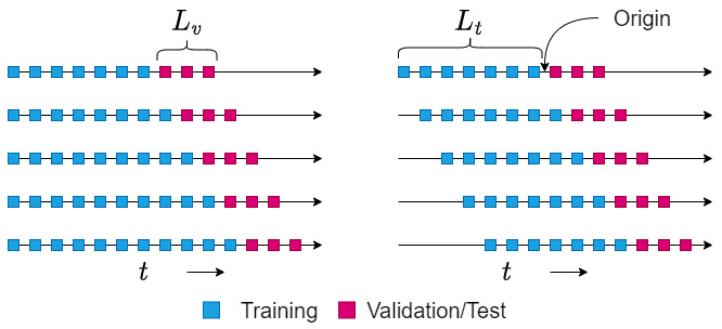
Figure 19.1 – Expanding (left) versus rolling (right) strategy

Under the expanding window strategy, the training split expands as the origin moves forward in time. In other words, under the expanding window strategy, we choose all the data that is available before the origin as the training split. This effectively increases the training length every time the origin moves forward in time.

In the rolling window strategy, we keep the length of the training split constant (). Therefore, when we move the origin forward by three timesteps, the training split drops three timesteps from the start of the time series.

Important note

Although the expanding and rolling window concept may remind you of the window we use for feature engineering or use as the context in deep learning models, this window is not the same. The window we talk about in this chapter is the window of training data that we chose to train our model. For instance, the features of a machine learning model may only extend to the 5 days before, and we can have the training split use the last 5 years of data.

There are merits and demerits to both of these window strategies. Let’s summarize them in a few key points:

• Expanding window is a good setup for a short time series, where the expanding window leads to more data being available for the models.
• Rolling window removes the oldest data from training. If the time series is non-stationary and the behavior is bound to change as time passes, having a rolling window will be beneficial to keep the model up to date.
• When we use the expanding window strategy for repeated evaluation, such as in cross-validation, the increase in time series length used for training can introduce some bias toward windows with a longer history. The rolling window strategy takes care of that bias by maintaining the same length of the series.

Calibration strategy

The calibration strategy is only valid in cases where we do multiple evaluations with different origins. There are two ways we can do evaluations with different origins – recalibrate every origin, or update every origin (terminology from Tashman, #1 in References).

Under the recalibrate strategy, the model is retrained with the new training split for every origin. This retrained model is used to evaluate the validation split. But, for the update strategy, we do not retrain the model, but use the trained model to evaluate the new validation split.

Let’s summarize a few key points to be considered for choosing a strategy here:

• The golden standard is to recalibrate every new origin, but many times this may not be feasible. In the econometrics/classical statistical models, the norm was to recalibrate every origin. That was feasible because those models are relatively less compute-intensive and the datasets at the time were also small. So, one could refit a model in a very short time. Nowadays, the datasets have grown in size, and so have the models. Retraining a deep learning model every time we move the origin may not be as easy.

Therefore, if you are using modern, complex models with long training times, an update strategy might be better.

• For classical models that run fast, we can explore the recalibration strategy.

But, if the time series you are forecasting is so dynamic that the behavior changes very frequently, then the recalibration strategy might be the way to go.

Now let’s get on to the third part of the validation strategy.

Sampling strategy

In the holdout strategy, we sample a point (origin) on the time series, preferably toward the end, such that the portion of the time series after the origin is shorter than the portion of the time series before. From this origin, we can use either the expanding or rolling window strategy to generate training and validation splits. The model is trained on the training split and tested on the held-out validation split. This strategy is simply called the holdout strategy. The calibration strategy is fixed at recalibrate because we are only testing and evaluating the model once.

The simple holdout strategy has one disadvantage – the forecast measure we have calculated on the held-out data may not be robust enough because of the single evaluation paradigm. We are relying on a single split of data to calculate the predictive performance of the model. For non-stationary series, this can be a problem because we might be selecting a model that captures the idiosyncrasies of the split that we have chosen.

We can get over this problem by repeating the holdout evaluation multiple times. We can either hand-tailor the different origins using business domain knowledge, such as taking into account seasonality, or some other factor. Or we could sample the origin points randomly. If we repeat this times, there will be validation splits, and they may or may not overlap with each other. The performance metric from these repeated trials can be aggregated using a function such as the mean, maximum, and minimum. This is called the repeated holdout (Rep-Holdout) strategy.

Note on implementation

The simple holdout strategy is very simple to implement because we decide the size of the validation split, and keep that much from the end of the time series aside as the validation. The Rep-Holdout strategy involves sampling multiple windows at random or using predefined windows as validation splits. We can make use of the PredefinedSplit class from scikit-learn to this effect.

Figure 19.2 shows the two holdout strategies using an expanding window approach:

Figure 19.2 – Holdout strategy (a) and Rep-Holdout strategy (b)

The Rep-Holdout strategy has a few more variants. The vanilla Rep-Holdout strategy evaluates multiple validation datasets, is mostly hand-crafted, and can have overlapping validation datasets. A variation of the Rep-Holdout strategy that insists that multiple validation splits should have no overlap is a more popular option. We call this Repeated Holdout (No Overlap) (Rep-Holdout-O). This has some properties from the cross-validation family and tries to use more data systematically. Figure 19.3(a) shows this strategy:

Figure 19.3 – Variations of Rep-Holdout strategy

The Rep-Holdout-O strategy is easy to implement in scikit-learn using the TimeSeriesSplit class for single time series datasets.

Notebook alert

The associated notebook that shows how to implement different validation strategies can be found in the Chapter19 folder under the name 01-Validation Strategies.ipynb.

The TimeSeriesSplit class from sklearn.model_selection implements the Rep-Holdout validation strategy and even supports expanding or rolling window variants. The main parameter is n_splits. This determines how many splits you want from the data, and the validation split size is decided automatically, according to this formula:

In the default configuration, this implements an expanding window Rep-Holdout-O strategy. But, there is a parameter, max_train_size. If we set this parameter, then it will use a window of max_train_size in a rolling window manner.

Yet another variant of the Rep-Holdout strategy introduces a gap of length between the train and validation splits. This is to increase the independence between the train and validation splits, hence getting a better error estimate through the procedure. We call this strategy Repeated Holdout (No Overlap) with Gaps (Rep-Holdout-O(G)). This strategy is depicted in Figure 19.3(b).

We can implement this using the TimeSeriesSplit class as well. All we need to do is use a parameter called gap. By default, the gap is set to 0. But if we change to a non-zero number, it inserts that much timestep gap between the end of the training and the beginning of validation.

Before we move on to the next set of strategies, let’s summarize and discuss some key points about the holdout strategies:

• Holdout strategies respect the temporal integrity of the problem and have been the preferred way of evaluating forecasting models for a long time.

But, it does have a weakness in the inefficient use of available data. For short time series, holdout or Rep-Holdout may not have enough training data to train a model.

• A simple holdout depends on a single evaluation, and the error estimate is not robust. Even in a stationary series, this procedure does not guarantee a good estimate of the error. In non-stationary time series, such as a seasonal time series, this problem exacerbates. But the Rep-Holdout and its variants take care of that issue.

Now let’s look at the other major school of thought.

Cross-validation strategies

Cross-validation is one of the most important tools when evaluating standard regression and classification methods. This is because of two reasons:

• A simple holdout approach doesn’t use all the data available and in cases where data is scarce, cross-validation makes the best use of the available data.
• Theoretically, the time series we have observed is one realization of a stochastic process, and so the acquired error measure of the data is also a stochastic variable. Therefore, it is essential to sample multiple error estimates to get an idea about the distribution of the stochastic variable. Intuitively, we can think of this as a “lack of reliability” on the error measure derived from a single slice of data.

The most common strategy that is used in standard machine learning is called k-fold cross-validation. Under this strategy, we randomly shuffle and partition the training data into k equal parts. Now, the whole training of the model and calculating the error is repeated k times, such that every k subset we have kept aside is used as a test set once, and only once. When we use a particular subset as testing data, we use all the other subsets as the training data. After we acquire k different estimates of the error measure, we aggregate it using a function such as an average. This mean will typically be more robust than a single error measure.

But, there is one assumption that is central to the validity procedure: i.i.d samples. This is one assumption that is invalid in time series problems because, by definition, the different samples in time series are dependent on each other through autocorrelation.

Additional information

Some argue that when we use time delay embedding to convert time series to a regression problem, we can start to use k-fold cross-validation on time series problems. While there are obvious theoretical problems, Bergmeir et al. (#2 in References) showed that empirically, the k-fold cross-validation is not a bad option. But, the caveat is that the time series needs to be stationary. We will talk more about this in the next section, where we will discuss the merits and demerits of these strategies.

But there have been modifications to the k-fold strategy, specifically aimed at sequential data.

Snijders et al. (#4 in References) proposed a modification we call the Blocked Cross-Validation (Bl-CV) strategy. It is similar to the standard k-fold strategy, but we do not randomly shuffle the dataset before partitioning into k subsets of length . So, this partitioning strategy results in k contiguous blocks of observations. Then, like a standard k-fold strategy, we train and test each of these k blocks and aggregate the error measure over these multiple evaluations. So, the temporal integrity of the problem is satisfied partially. In other words, temporal integrity is maintained within each of the blocks, but not between the blocks. Figure 19.4(a) shows this strategy:

Figure 19.4 – Bl-CV strategies

To implement the Bl-CV strategy, we can use the same Kfold class from scikit-learn. As we saw earlier, the main parameter the cross-validation classes in scikit-learn takes in is n_splits. Here, n_splits also defines the number of equally sized folds it selects. There is another parameter, shuffle, which is set to True by default. If we make sure our data is sorted according to time, then use the Kfold class with shuffle=False, it will imitate the Bl-CV strategy. The associated notebook shows this usage. I urge you to check the notebook for a better understanding of how this is implemented.

In the previous section, we talked about introducing gaps between train and validation splits, to increase independence between them. Another variant of the Bl-CV is a version that uses these gaps. We call it Blocked Cross-Validation with Gaps (Bl-CV(G)). We can see this in action in Figure 19.4(b).

Unfortunately, the Kfold implementation in scikit-learn does not support this variant. But, it’s simple to extend the Kfold implementation to include gaps as well. The associated notebook has an implementation of this. It has an additional parameter, gap, that lets us set the gap between the train and validation splits.

We saw many different strategies for validation; now let’s try and lay down a few points that will help you in deciding the right strategy for your problem.

Choosing a validation strategy

Choosing the right validation strategy is one of the most important, but overlooked tasks in the machine learning workflow. A good validation setup will go a long way in all the different steps in the modeling process, such as feature engineering, feature selection, model selection, and hyperparameter tuning. Although there are no hard and fast rules in setting up a validation strategy, there are a few guidelines we can follow. Some of them are from experience (both mine and others) and some of them are from empirical and theoretical studies that have been published as research papers:

• One guiding principle in the design is that we try to make the validation strategy replicate the real use of the model as much as possible. For instance, if the model is going to be used to predict the next 24 timesteps, we make the length of the validation split 24 timesteps. Of course, it’s not as simple as that, because other practical constraints such as the availability of enough data, time, and computers have to be kept in mind while designing a validation strategy.
• Rep-Holdout strategies that respect the temporal order of the time series problem are the preferred option, especially in cases where there is sufficient data available.
• For purely autoregressive formulations of stationary time series, regular Kfold can also be used and Bergmeir et al. (#2 in References) empirically show that they perform better than holdout strategies. But, Blocked Cross Validation is a better alternative among cross-validated strategies. Cerqueira et al. (#3 in References) corroborated the findings in their empirical study for stationary time series.
• If the time series is non-stationary, then Cerqueira et al. showed empirically that the holdout strategies (especially Rep-Holdout strategies) are the best ones to choose.
• If the time series is short, using Bl-CV after making the time series stationary is a good strategy for autoregressive formulations, such as time delay embedding. But, for models that use some kind of memory of the history to forecast, such as exponential smoothing or deep learning models such as RNN, cross-validation strategies may not be safe to use.
• If we have exogenous variables, in addition to the autoregressive part, it may not be safe to use cross-validation strategies. It is best to stick to holdout-based strategies.
• For a strongly seasonal time series, it is beneficial to use validation periods that mimic the forecast horizon. For instance, if we are forecasting for October, November, and December, it is beneficial to check the performance of the model in October, November, and December of last year.

Up until now, we were talking about validation strategies for a single time series. But in the context of global models, we are at a point where we need to think about validation strategies for such cases as well.

Validation strategies for datasets with multiple time series

All the strategies we have seen till now are perfectly valid for datasets with multiple time series, such as the London Smart Meters dataset we have been working with in this book. The insights we discussed in the last section are also valid. The implementation of such strategies can be slightly tricky because the scikit learn classes we discussed work for single time series. Those implementations assume that we have a single time series, sorted according to the temporal order. If there are multiple time series, the splits will be haphazard and messy.

There are a couple of options we can adopt for datasets with multiple time series:

• We can loop over the different time series and use the methods we discussed to do the train-validation split, and then concatenate the resulting sets across all the time series. But, that is not going to be so efficient.
• We can write some code and design the validation strategies to use datetime or a time index (such as the one we saw in PyTorch forecasting in Chapter 15, Strategies for Global Deep Learning Forecasting Models). I have linked to a brilliant notebook from Konrad Banachewicz in the Further reading section of this chapter, where he uses a custom GroupSplit class that uses the time index as the group. This is one way to use Rep-Holdout strategies on a dataset with multiple time series.

There are a few points that we need to keep in mind for datasets with multiple time series:

• Do not use different time windows for different time series. This is because different windows in time would have different errors, and that would skew the aggregate error metric we are tracking.
• If different time series have different lengths, align the length of the validation period across all the series. Training length can be different, but validation windows should be the same so that every time series equally contributes to the aggregate error metric.
• It is easy to get carried away by complicated validation schemes, but always keep the technical debt you incur by choosing a specific technique in mind.

With that, we have come to the end of a short but important chapter.

Summary

We have come to the end of our journey through the world of time series forecasting. In the last couple of chapters, we addressed a few mechanics of forecasting, such as how to do multi-step forecasting, and how to evaluate forecasts. Different validation strategies for evaluating forecasts and forecasting models were the topics of the current chapter. We started by enlightening you as to why model validation is an important task. Then, we looked at a few different validation strategies, such as the holdout strategies, and navigated the controversial use of cross-validation for time series. We spent some time summarizing and laying down a few guidelines to be used to select a validation strategy. To top it all off, we looked at how these validation strategies are applicable to datasets with multiple time series and talked about how to adapt them to such scenarios.

With that, we have come to the end of the book. Congratulations on making it all the way through, and I hope you have gained enough skills from the book to tackle the next time series problem that comes your way. I strongly urge you to start putting into practice the skills that you have gained from the book because, as Richard Feynman rightly put it, "You do not know anything until you have practiced."

References

The following are the references used in this chapter:

1. Tashman, Len. (2000). Out-of-sample tests of forecasting accuracy: An analysis and review. International Journal of Forecasting. 16. 437-450. 10.1016/S0169-2070(00)00065-0: https://www.researchgate.net/publication/223319987_Out-of-sample_tests_of_forecasting_accuracy_An_analysis_and_review
2. Bergmeir, Christoph and Benítez, José M. (2012). On the use of cross-validation for time series predictor evaluation. In Information Sciences, Volume 191, 2012, Pages 192-213: https://www.sciencedirect.com/science/article/abs/pii/S0020025511006773
3. Cerqueira, V., Torgo, L., and Mozetič, I. (2020). Evaluating time series forecasting models: an empirical study on performance estimation methods. Mach Learn 109, 1997–2028 (2020): https://doi.org/10.1007/s10994-020-05910-7
4. Snijders, T.A.B. (1988). On Cross-Validation for Predictor Evaluation in Time Series. In: Dijkstra, T.K. (eds) On Model Uncertainty and its Statistical Implications. Lecture Notes in Economics and Mathematical Systems, vol 307. Springer, Berlin, Heidelberg. https://doi.org/10.1007/978-3-642-61564-1_4

Further reading

TS-10: Validation methods for time series by Konrad Banachewicz – https://www.kaggle.com/code/konradb/ts-10-validation-methods-for-time-series