Applications based on Natural Language Processing (NLP) have witnessed a tremendous rise in the last few years. New use cases are coming along every day and in order to keep pace with the ever-evolving demand, the need of the hour is to research, innovate, and build efficient solutions for solving the complex problems we face. Innovation in the field of NLP over the years has made it possible to solve some of the most challenging problems, such as language translation and building chatbots, among others.

In this chapter, we will take a look at some of the recent advancements in the field of NLP. We will begin by developing an understanding of Sequence-to-Sequence (Seq2Seq) models and discuss encoders and decoders in the process. We will use this new knowledge to build a French-to-English translator using Seq2Seq modeling. After that, we will have a look at the attention mechanism, one of the key recent developments. The attention mechanism has not only improved the inferencing abilities of existing architectures but has also paved the way for the development of other amazingly efficient architectures such as Transformers and Bidirectional Encoder Representations from Transformers (BERT), which we will look at toward the end of this chapter.

The following topics will be covered in this chapter:

• Seq2Seq modeling
• Translating between languages using Seq2Seq modeling
• Let's pay some attention
• Transformers
• BERT

Technical requirements

The code files for this chapter can be found at the following GitHub link: https://github.com/PacktPublishing/Hands-On-Python-Natural-Language-Processing/tree/master/Chapter11.

Seq2Seq modeling

Before we begin with Seq2Seqmodeling, I would like to share an anecdote that I witnessed at Bengaluru Airport in India. A traveler from China was trying to order a meal at one of the airport restaurants and the butler was unable to comprehend Mandarin. An onlooker stepped in and used Google Translate to convert the English being spoken by the store owner into Mandarin and vice versa. Seq2Seq modeling has helped build applications such as Google Translate, which made the conversation between these folks possible.

When we try to build chatbots or language translating systems, we essentially try to convert a sequence of text of some arbitrary length into another sequence of text of some unknown length. For example, the same chatbot might respond with one word or multiple words depending on the conversational prompts coming from the other party involved in the conversation. We do not always respond with text of the same length. We saw this as one of the many-to-many variants of the RNN architecture in Chapter 10, Capturing Temporal Relationships in Text. This architecture is referred to as Seq2Seq modeling, where we try to convert one sequence into another.

Let's consider the example of language translation.

The English sentence how are you doing? is written as como estas? in Spanish. These two sentences are of different lengths. Let's think of another example: can we do this? in English is represented as podemos hacer esto? in Spanish. Even though both English sentences have four words in them, their Spanish counterparts are of differing lengths. When building such systems, we try to map an input sequence to an output sequence that can be of varying lengths.

Okay. Now that we understand what Seq2Seq modeling is, how do we do it? We use two building blocks, called Encoders and Decoders and shown in the following diagram, to build our Seq2Seq modeling systems:

These encoders and decoders can be built using Long Short Term Memory (LSTM) networks, Gated Recurrent Units (GRU), and so on. Let's take a deep dive and understand how these encoders and decoders enable us to build these systems.

Encoders

The encoder is the first component in the encoder-decoder architecture. The input data is fed to the encoder and it builds a representation of the input data. This low-dimensional representation of the input data is referred to as the context vector. Some literature also refers to it as the thought vector. The context vector tries to capture the meaning in the input data. Essentially, it tries to build an embedding for the input data.

The encoder can be built using RNNs, LSTMs, GRUs, or bidirectional RNNs, among others. We saw that RNN-based architectures hold the context of the inputs that they saw in the hidden state. Hence, the last hidden state will hold the context of the entire sentence. The hidden state from the last timestep is what we want. It is our context vector since it has seen all the input and has maintained the context of all the input words.

Let's think of a natural language translation task where we want to convert sentences from English into French. As an example, let's pick the sentence, Learning Natural Language Processing and see what the encoder does to convert it into its French equivalent:

The preceding diagram illustrates an encoder built using LSTM that develops a context vector for the English sentence, Learning Natural Language Processing. The output from the encoder is the context vector, which contains two parts:

• The hidden state from the last timestep of the encoder
• The memory state of the LSTM for the input sentence

Now that we have successfully built a context vector of our input sentence, the next step is to decode this context vector and build our French sentence using it. Let's do that next.

Decoders

We got an embedding of our input sentence, Learning Natural Language Processing, using the encoder. The next part is to decode this context vector and build its French representation, Apprendre le traitement du langage naturel. The following diagram shows how a decoder, built using LSTM, gets trained to do this:

Let's understand its working in depth next.

Up to now, we have seen that the initial hidden state for any RNN-based architecture is a randomly initialized vector. However, with decoders, the input is the context vector that we received as output from the encoder.

Okay, we have now understood that the initial hidden state should not be a randomly initialized vector, but rather, the context vector. However, we still don't understand what the input to the decoder should be.

The input to the decoder at the first timestep is a token that indicates the start of the sentence,<start>. Using this <start> token, the decoder now has the task of learning to predict the first token of the target sentence. However, the working of the decoder is a little different for the learning and inferencing phases explained next. Let's understand that now.

The training phase

During the training phase, the decoder has passed the target sequence as input along with the context vector. The input to the decoder at timestep 0 is the <start> token. At timestep 1 the input to the decoder is the predicted token or the first token of the target sequence, and so on. The decoder's job here is to learn that when provided a context vector and an initial <start> token, it should be capable of producing a set of tokens.

The inference phase

During the inference stage, we don't know what the target sequence should be and it is the decoder's job to predict this target sequence. The decoder will receive the context vector and the initial token using which it should be able to predict the first token. Thereon, it should be able to predict the second token, using the first predicted token and the hidden state from the first timestep, and this should continue as such. Essentially, the input at timestep t is the predicted output of the previous timestep t-1, as shown in the diagram in the Decoders section. The input at timestep 1 is Apprendre, which is actually the predicted output from the previous timestep. The same pattern follows for the rest of the decoder's work.

Okay, we've got a fair idea of the initial hidden state and also how the decoder learns and predicts, but we need to stop sending outputs at the point when predictions occur. How do we do that?

Whenever the output from a decoder state is a token indicating the end of the sentence, <end>, or we have reached a pre-defined maximum length of output or target sequence, we get a signal that the decoder has completed its job of building the output sequence and we need to stop here.

Simple LSTMs on both ends enabled us to convert one sequence of data to another using just a context vector in between them. This approach for Seq2Seq generation can be used to build chatbots, speech recognition systems, natural language translation systems, and so on. Now that we have a sound theoretical understanding of Seq2Seq generation systems, let's try and do some practical stuff with it in the next section.

Translating between languages using Seq2Seq modeling

English is the most spoken language in the world and French is an official language in 29 countries. As part of this exercise, we will build a French-to-English translator. Let's begin:

1. As with any other exercise, we begin by importing the libraries that we need to build our French-to-English translator:

import pandas as pd
import string
import re
import io
import numpy as np
from unicodedata import normalize
import keras, tensorflow
from keras.models import Model
from keras.layers import Input, LSTM, Dense

2. Now that we have imported our libraries, let's read the dataset using the following code block:

def read_data(file):
    data = []
    with io.open(file, 'r') as file:
        for entry in file:
            entry = entry.strip()
            data.append(entry)
    return data
data = read_data('dataset/bilingual_pairs.txt')

3. Let's figure out some basics of our data.

We can see some of the data points using the following code block:

data[139990:140000]

Here's the output:

['Never choose a vocation just because the hours are short.	Ne choisissez jamais une profession juste parce que les heures y sont courtes.',
 "No other mountain in the world is so high as Mt. Everest.	Aucune montagne au monde n'atteint la hauteur du Mont Everest.",
 "No sooner had he met his family than he burst into tears.	À peine avait-il rencontré sa famille qu'il éclata en sanglots.",
 "Nothing is more disappointing than to lose in the finals.	Rien n'est plus décevant que de perdre en finale.",
 "Now that he is old, it is your duty to go look after him.	À présent qu'il est vieux, c'est ton devoir de veiller sur lui.",
 "Now that you've decided to quit your job, you look happy.	Maintenant que vous avez décidé de quitter votre emploi, vous avez l'air heureux.",
 "Now that you've decided to quit your job, you look happy.	Maintenant que tu as décidé de quitter ton emploi, tu as l'air heureux.",
 "Now that you've decided to quit your job, you look happy.	Maintenant que vous avez décidé de quitter votre emploi, vous avez l'air heureuse.",
 "Now that you've decided to quit your job, you look happy.	Maintenant que tu as décidé de quitter ton emploi, tu as l'air heureuse.",
 'Please drop in when you happen to be in the neighborhood.	Veuillez donc passer quand vous êtes dans le coin !']

The output shows that our data consists of tab-separated English-French sentence pairs.

Let's see the size of our dataset next:

len(data)

The size of our data is as follows:

145437

We use the first 140,000 English-French sentence pairs for this exercise:

data = data[:140000]

4. We saw that our dataset contains tabs that separate the English-French sentence pairs, so we need to split them into different English and French lists:

def build_english_french_sentences(data):
    english_sentences = []
    french_sentences = []
    for data_point in data:
        english_sentences.append(data_point.split("	")[0])
        french_sentences.append(data_point.split("	")[1])
    return english_sentences, french_sentences
english_sentences, french_sentences = build_english_french_sentences(data)

5. Now that we have different lists holding our English and French sentences, let's clean our data next.

The clean_sentence method defined in the following code block takes care of processing individual sentences:

def clean_sentences(sentence):
    # prepare regex for char filtering
    re_print = re.compile('[^%s]' % re.escape(string.printable))
    # prepare translation table for removing punctuation
    table = str.maketrans('', '', string.punctuation)
    cleaned_sent = normalize('NFD', sentence).encode('ascii', 
                                                     'ignore')
    cleaned_sent = cleaned_sent.decode('UTF-8')
    cleaned_sent = cleaned_sent.split()
    cleaned_sent = [word.lower() for word in cleaned_sent]
    cleaned_sent = [word.translate(table) for word in cleaned_sent]
    cleaned_sent = [re_print.sub('', w) for w in cleaned_sent]
    cleaned_sent = [word for word in cleaned_sent if 
                    word.isalpha()]
    return ' '.join(cleaned_sent)

The previous function does the following:

• Normalizes characters
• Removes punctuation
• Performs case-folding
• Removes non-printable characters
• Keeps only alphabetic words

Next, we will build a function, build_clean_english_french_sentences(), and get it to clean our English and French sentences by calling the function we defined in the previous code block on individual sentences:

def build_clean_english_french_sentences(english_sentences, french_sentences):
    french_sentences_cleaned = []
    english_sentences_cleaned = []
    for sent in french_sentences:
        french_sentences_cleaned.append(clean_sentences(sent))
    for sent in english_sentences:
        english_sentences_cleaned.append(clean_sentences(sent))
    return english_sentences_cleaned, french_sentences_cleaned

english_sentences_cleaned, french_sentences_cleaned = build_clean_english_french_sentences(english_sentences, french_sentences)

6. We cleaned our data in the previous step. The following steps are where we build our vocabulary and also add tokens that convey the start and end of a sequence, as required by our decoder.

In Chapter 10, Capturing Temporal Relationships in Text, when we had built a text generator, we used words as our vocabulary. However, we will go down to the character level in order to build our vocabulary in this exercise, as defined in the following code block:

def build_data(english_sentences_cleaned, french_sentences_cleaned):
    input_dataset = []
    target_dataset = []
    input_characters = set()
    target_characters = set()

    for french_sentence in french_sentences_cleaned:
        input_datapoint = french_sentence
        input_dataset.append(input_datapoint)
        for char in input_datapoint:
            input_characters.add(char)

    for english_sentence in english_sentences_cleaned:
        target_datapoint = "	" + english_sentence + "
"
        target_dataset.append(target_datapoint)
        for char in target_datapoint:
            target_characters.add(char)

    return input_dataset, target_dataset, 
           sorted(list(input_characters)), 
           sorted(list(target_characters)) 

input_dataset, target_dataset, input_characters, target_characters = build_data(english_sentences_cleaned, french_sentences_cleaned)

The method defined in the previous code block helped us to do the following:

• Add to our target data to convey the start of a sentence to our decoder.
• Add to our target data to convey the end of a sentence to our decoder.
• Prepare a list of unique input and output characters. Our model will try and predict at the character level for this exercise.

7. We developed our input and target vocabularies in the previous step. Let's see what unique input and output characters are in store for us with the following command:

print(input_characters)

Here's our set of input characters:

[' ', 'a', 'b', 'c', 'd', 'e', 'f', 'g', 'h', 'i', 'j', 'k', 'l', 'm', 'n', 'o', 'p', 'q', 'r', 's', 't', 'u', 'v', 'w', 'x', 'y', 'z']

Next, let's see our target characters with the following command:

print(target_characters)

Here's our set of target characters:

['	', '
', ' ', 'a', 'b', 'c', 'd', 'e', 'f', 'g', 'h', 'i', 'j', 'k', 'l', 'm', 'n', 'o', 'p', 'q', 'r', 's', 't', 'u', 'v', 'w', 'x', 'y', 'z']

Notice that in addition to our input characters, the target character dataset has and tokens, which help the decoder to understand the start and end of a target sequence.

8. Our input and output vocabulary may not be the same for tasks such as natural language translation. In fact, at times, our character set may not be the same either. For example, we might be trying to translate between English and Hindi, which have different character sets altogether.

Apart from the difference in vocabulary, we should also be aware that our input sequence and target sequence may not be of the same size.

The English sentence how are you today, dear? is written in French as comment tu vas aujourd'hui mon cher.

The number of words in the preceding sentences is different. If we go to the character level, then we can see that the number of characters in both sentences is very different as well.

Let's take another very similar English sentence, how are you today? which is written in French as comment vas-tu aujourd'hui? Now, if we make a comparison between the two examples we discussed, their English and French counterparts have differing lengths.

We next want to find out some metadata about our data, in terms of the following:

• The size of the input and target vocabularies (basically, the size of the input and target character sets)
• The maximum length of input and output character sequences

The following code block helps us to do that:

def build_metadata(input_dataset, target_dataset, 
                   input_characters, target_characters):    
    num_Encoder_tokens = len(input_characters)
    num_Decoder_tokens = len(target_characters)
    max_Encoder_seq_length = max([len(data_point) for data_point 
                                  in input_dataset]) 
    max_Decoder_seq_length = max([len(data_point) for data_point 
                                  in target_dataset])
    print('Number of data points:', len(input_dataset))
    print('Number of unique input tokens:', num_Encoder_tokens)
    print('Number of unique output tokens:', num_Decoder_tokens)
    print('Maximum sequence length for inputs:', 
           max_Encoder_seq_length)
    print('Maximum sequence length for outputs:', 
           max_Decoder_seq_length)
    return num_Encoder_tokens, num_Decoder_tokens, 
           max_Encoder_seq_length, max_Decoder_seq_length

num_Encoder_tokens, num_Decoder_tokens, max_Encoder_seq_length, max_Decoder_seq_length = build_metadata(input_dataset, target_dataset, input_characters, target_characters)

Here's the metadata we acquired using the previous code block:

Number of data points: 140000
Number of unique input tokens: 27
Number of unique output tokens: 29
Maximum sequence length for inputs: 117
Maximum sequence length for outputs: 58

Here's what we get from the metadata:

• We have 140,000 unique English-French sentence pairs in our dataset.
• The number of unique input tokens/characters is 27.
• The number of unique target tokens/characters that we'll try and predict is 29.
• Our longest input character sequence is 117 characters long.
• Our longest target character sequence is 58 characters long.

9. A very important step is to build mappings from characters to indices and vice versa. This will help us to do the following:

• Represent our input characters using their corresponding indices
• Convert our predicted indices into their corresponding characters when making predictions

The following code block helps us with this:

def build_indices(input_characters, target_characters):
    input_char_to_idx = {}
    input_idx_to_char = {}
    target_char_to_idx = {}
    target_idx_to_char = {}

    for i, char in enumerate(input_characters):
        input_char_to_idx[char] = i
        input_idx_to_char[i] = char

    for i, char in enumerate(target_characters):
        target_char_to_idx[char] = i
        target_idx_to_char[i] = char

    return input_char_to_idx, input_idx_to_char, 
           target_char_to_idx, target_idx_to_char

input_char_to_idx, input_idx_to_char, target_char_to_idx, target_idx_to_char = build_indices(input_characters, target_characters)

10. Next, we build our data structure based on the metadata we obtained in step 8 using the following code block:

def build_data_structures(length_input_dataset, max_Encoder_seq_length, max_Decoder_seq_length, num_Encoder_tokens, num_Decoder_tokens):

    Encoder_input_data = np.zeros((length_input_dataset, 
      max_Encoder_seq_length, num_Encoder_tokens), dtype='float32')
    Decoder_input_data = np.zeros((length_input_dataset, 
      max_Decoder_seq_length, num_Decoder_tokens), dtype='float32')
    Decoder_target_data = np.zeros((length_input_dataset, 
      max_Decoder_seq_length, num_Decoder_tokens), dtype='float32')
    print("Dimensionality of Encoder input data is : ", 
           Encoder_input_data.shape)
    print("Dimensionality of Decoder input data is : ", 
           Decoder_input_data.shape)
    print("Dimensionality of Decoder target data is : ", 
           Decoder_target_data.shape)
    return Encoder_input_data, Decoder_input_data, 
           Decoder_target_data

Encoder_input_data, Decoder_input_data, Decoder_target_data = build_data_structures(len(input_dataset), max_Encoder_seq_length, max_Decoder_seq_length, num_Encoder_tokens, num_Decoder_tokens)

Here's the output that shows the shape of the data structures we built:

• The dimensionality of the encoder input data is (140000, 117, 27).
• The dimensionality of the decoder input data is (140000, 58, 29).
• The dimensionality of the decoder target data is (140000, 58, 29).

Note the following points:

• The dimensionality of the input data is (140000, 117, 27):
• The first dimension caters to the number of data points we have: 140,000.
• The second dimension caters to the maximum length of our input sequence: 117.
• The third dimension caters to the number of unique inputs we can have or the size of our input character set: 27.
• The dimensionality of the decoder input and decoder target data is (140000, 58, 29):
• The first dimension caters to the number of data points we have: 140,000.
• The second dimension caters to the maximum length of our target sequence: 58.
• The third dimension caters to the number of unique inputs we can have or the size of our target character set: 29.

11. Now that we have our data structure ready, it is time to add some data to it:

def add_data_to_data_structures(input_dataset, target_dataset, Encoder_input_data, Decoder_input_data, Decoder_target_data):
    for i, (input_data_point, target_data_point) in 
            enumerate(zip(input_dataset, target_dataset)):
        for t, char in enumerate(input_data_point):
            Encoder_input_data[i, t, input_char_to_idx[char]] = 1.
        for t, char in enumerate(target_data_point):
            # Decoder_target_data is ahead of Decoder_input_data by 
            # one timestep
            Decoder_input_data[i, t, target_char_to_idx[char]] = 1.
            if t > 0:
                # Decoder_target_data will be ahead by one timestep
                # and will not include the start character.
                Decoder_target_data[i, t - 1, 
                                    target_char_to_idx[char]] = 1.
    return Encoder_input_data, Decoder_input_data, 
           Decoder_target_data

Encoder_input_data, Decoder_input_data, Decoder_target_data = add_data_to_data_structures(input_dataset, target_dataset, Encoder_input_data, Decoder_input_data, Decoder_target_data)

We have used the character-to-indices mapping and converted some entries in our data structure to 1, which indicates the presence of a particular character at a specific position in each of the sentences.

If you carefully examine our work so far, notice that the last dimension (27 in the encoder input data structure and 29 in the decoder input or decoder target) is a one-hot vector, which indicates which entry is present for that particular position in our data.

One final thing to note is that when building the decoder target data, we do not include anything for the <start> token, and it is also ahead by one timestep for the same reasons that we discussed when talking about decoders in the previous section.

Our decoder target data is the same as the decoder input data, except that it is offset by one timestep.

12. We are ready with our data, so let's define the hyperparameters for our model:

batch_size = 256
epochs = 100
latent_dim = 256

13. It's time we bring our encoder into existence using the following code block:

Encoder_inputs = Input(shape=(None, num_Encoder_tokens))
Encoder = LSTM(latent_dim, return_state=True)
Encoder_outputs, state_h, state_c = Encoder(Encoder_inputs)
Encoder_states = [state_h, state_c]

We have set return_ state as True so that the decoder returns us the last hidden state and memory, which will form the context vector.

state_h and state_c represent our last hidden state and memory cell, respectively.

However, how does our encoder learn?

The encoder's job is to provide a context vector where it captures the context or thought in the input sentence. However, we do not have any explicit target context vector defined against which to compare the encoder's performance. The encoder learns from the performance of the decoder, which happens further down the line. The decoder's error flows back and that's how the backpropagation in the encoder works and it learns.

14. Let's define the second part of our architecture, the decoder, using the following code block:

Decoder_inputs = Input(shape=(None, num_Decoder_tokens))
Decoder_lstm = LSTM(latent_dim, return_sequences=True, 
                    return_state=True)
Decoder_outputs, _, _ = Decoder_lstm(Decoder_inputs, 
                        initial_state=Encoder_states)
Decoder_dense = Dense(num_Decoder_tokens, activation='softmax')
Decoder_outputs = Decoder_dense(Decoder_outputs)

As we discussed, during training, the decoder is provided both the input data and the target data and is asked to predict the input data with an offset of 1. This helps the decoder to understand, given a context vector from the encoder, what it should be predicting. This method of learning is referred to as teacher forcing.

The initial state for the decoder is Encoder_states, which is our context vector retrieved from the encoder in step 13.

A dense layer is part of the decoder where the number of neurons is equal to the number of tokens (characters in our case) present in the decoder's target character set. The dense layer is coupled with the softmax output that helps us to get the normalized probabilities for every target character. It predicts the target character with the highest probability.

The return_sequences parameter in the decoder LSTM helps us to retrieve the entire output sequence from the decoder. We want an output from the decoder at every timestep and that is why we set this parameter to True. Since we used the dense layer along with the softmax output, we get a probability distribution over our target characters for every timestep, and as mentioned already, we pick the character with the highest probability. We judge the performance of our decoder by comparing its output produced at every timestep.

15. We have defined our encoder and decoder, but how do they come together to build our model? The way we define our model here will be a little different from what we had in our previous examples. We use the Keras Model API to define the various inputs and outputs we will use at various stages. The Model API is provided by Encoder_input_data; Decoder_input_data is the input to our model, which will be used as the encoder and decoder inputs; and Decoder_target_data is used as the decoder output. The model will try to convert Encoder_input_data and Decoder_input_data into Decoder_target_data:

model = Model(inputs=[Encoder_inputs, Decoder_inputs], outputs=Decoder_outputs)

Let's compile and train our model next:

model.compile(optimizer='rmsprop', loss='categorical_crossentropy')
model.summary()

Here's the summary of our model:

Model: "model_1"
__________________________________________________________________________________________________
Layer (type)                    Output Shape         Param #     Connected to                     
==================================================================================================
input_1 (InputLayer)            (None, None, 27)     0                                            
__________________________________________________________________________________________________
input_2 (InputLayer)            (None, None, 29)     0                                            
__________________________________________________________________________________________________
lstm_1 (LSTM)                   [(None, 256), (None, 290816      input_1[0][0]                    
__________________________________________________________________________________________________
lstm_2 (LSTM)                   [(None, None, 256),  292864      input_2[0][0]                    
                                                                 lstm_1[0][1]                     
                                                                 lstm_1[0][2]                     
__________________________________________________________________________________________________
dense_1 (Dense)                 (None, None, 29)     7453        lstm_2[0][0]                     
==================================================================================================
Total params: 591,133
Trainable params: 591,133
Non-trainable params: 0

Let's train our model now:

model.fit([Encoder_input_data, Decoder_input_data], 
          Decoder_target_data, 
          batch_size=batch_size,
          epochs=epochs,
          validation_split=0.2)

We train on 80% of our data and validate on the remaining 20% of the data.

Here's some sample output from our model training:

Train on 112000 samples, validate on 28000 samples
Epoch 1/100
112000/112000 [==============================] - 114s 1ms/step - loss: 0.9022 - val_loss: 1.5125
Epoch 2/100
112000/112000 [==============================] - 115s 1ms/step - loss: 0.7103 - val_loss: 1.3070
Epoch 3/100
112000/112000 [==============================] - 115s 1ms/step - loss: 0.6220 - val_loss: 1.2398
Epoch 4/100
112000/112000 [==============================] - 116s 1ms/step - loss: 0.5705 - val_loss: 1.1785
Epoch 5/100
112000/112000 [==============================] - 116s 1ms/step - loss: 0.5368 - val_loss: 1.1203
Epoch 6/100
112000/112000 [==============================] - 116s 1ms/step - loss: 0.5117 - val_loss: 1.1075
Epoch 7/100
112000/112000 [==============================] - 115s 1ms/step - loss: 0.4921 - val_loss: 1.1037
Epoch 8/100
112000/112000 [==============================] - 114s 1ms/step - loss: 0.4780 - val_loss: 1.0276

16. We save our model next using the following code:

model.save('Output Files/neural_machine_translation_french_to_english.h5')

17. Hey! Are we done? We trained our model to convert a French sentence into English. However, we did not figure out how we would infer from the model we built.

We do this with the following code block. This performs the following steps:

1. We send the input sequence to the encoder and retrieve the initial decoder state.
2. After this, we send the start token ( in our case) and the initial decoder state to the decoder to get the next target character as the output.
3. We then add the predicted target character to the sequence.
4. Repeat from step 2 until we obtain the end token or reach the maximum number of predicted characters:

Encoder_model = Model(Encoder_inputs, Encoder_states)

Decoder_state_input_c = Input(shape=(latent_dim,))
Decoder_state_input_h = Input(shape=(latent_dim,))
Decoder_states_inputs = [Decoder_state_input_h, 
                         Decoder_state_input_c]

Decoder_outputs, state_h, state_c = Decoder_lstm(Decoder_inputs, 
                                initial_state=Decoder_states_inputs)
Decoder_states = [state_h, state_c]
Decoder_outputs = Decoder_dense(Decoder_outputs)

Decoder_model = Model([Decoder_inputs] + Decoder_states_inputs,
                      [Decoder_outputs] + Decoder_states)

Let's define the decode_sequence() method that uses the encoder-decoder model we built:

def decode_sequence(input_seq):

    states_value = Encoder_model.predict(input_seq)

    target_seq = np.zeros((1, 1, num_Decoder_tokens))
    target_seq[0, 0, target_char_to_idx['	']] = 1.

    stop_condition = False
    decoded_sentence = ''
    while not stop_condition:
        output_tokens, h, c = Decoder_model.predict([target_seq]+ 
                                                     states_value)

        sampled_token_index = np.argmax(output_tokens[0, -1, :])
        sampled_char = target_idx_to_char[sampled_token_index]
        decoded_sentence += sampled_char

        if (sampled_char == '
' or len(decoded_sentence) > 
            max_Decoder_seq_length):
              stop_condition = True


        target_seq = np.zeros((1, 1, num_Decoder_tokens))
        target_seq[0, 0, sampled_token_index] = 1.

        states_value = [h, c]

    return decoded_sentence

A simple call to the decode_ sequence() method defined in the preceding code will help us with our inference.

18. Let's translate some French to English now:

def decode(seq_index):
    input_seq = Encoder_input_data[seq_index: seq_index + 1]
    decoded_sentence = decode_sequence(input_seq)
    print('-')
    print('Input sentence:', input_dataset[seq_index])
    print('Decoded sentence:', decoded_sentence)

Let's make a few calls to the decode method to perform our translations. The decode method takes in the index of a French data point and converts it into English.

Let's decode the 55,000^th French sentence from our data first:

decode(55000)

Here's the output:

Input sentence: hier etait une bonne journee
Decoded sentence: yesterday was a little too far

The next call will decode the 10,000^th sentence:

decode(10000)

Here's the output:

Input sentence: jen ai ras le bol
Decoded sentence: im still not sure

The next method call decodes the 200^th sentence:

decode(200)

Here's the output:

Input sentence: soyez calmes
Decoded sentence: be careful

Let's decode the 3,000^th sentence next:

decode(3000)

Here's the output:

Input sentence: je me sens affreusement mal
Decoded sentence: i feel like such an idiot

We will decode the 40,884^th sentence next:

decode(40884)

Here's the output:

Input sentence: je pense que je peux arranger ca
Decoded sentence: i think i can do it

Comparisons with Google Translate results showed that our model performs a decent job. Also, the output contains proper English words. However, we have only tried to decode sentences from the input data.

The model can further be built at the word level instead of training it at the character level, as we did in this exercise.

We can try tuning our hyperparameters and see if we make improvements with our translation results.

Now that we have successfully built a Seq2Seq model, in the upcoming sections, let's understand some more architectures that were developed in the recent past.

Let's pay some attention

The encoder-decoder architecture that we studied in the previous section for neural machine translation converted our source text into a fixed-length context vector and sent it to the decoder. The last hidden state was used by our decoder to build the target sequence.

Research has shown that this approach of sending the last hidden state turns out to be a bottleneck for long sentences, especially where the length of the sentence is longer than the sentences used for training. The context vector is not able to capture the meaning of the entire sentence. The performance of the model is not good and keeps deteriorating in such cases.

A new mechanism called the attention mechanism,shown in the following diagram,evolved to solve this problem of dealing with long sentences. Instead of sending only the last hidden state to the decoder, all the hidden states are passed on to the decoder. This approach provides the ability to encode an input sequence into a sequence of vectors without being constrained to a single fixed-length vector as was the case earlier. The network is now freed from having to use a single vector to represent all the information in the source sequence. During the decoding stage, these sequences of vectors are weighted at every timestep to figure out the relevance of each input for predicting a particular output. This does not mean a one-to-one mapping between the input token and output token. The target word is predicted during the decoding stage using the sum of the weighted context hidden states along with the previous target words:

Let's understand in depth how the attention mechanism works. The computation of the context vector is performed using the following steps:

1. The first step is to obtain the hidden states, as shown in the following diagram:

2. Now we have the decoder hidden state vector d. Each of the encoder's hidden state vectors, along with the decoder hidden state vector, are passed to a function such as a dot product, as shown in the following diagram. The function returns a score for each of these input hidden states for that particular timestep t. This score reflects the importance of the various input tokens toward the prediction of the token at timestep t:

The following shows some example attention scores for each of the hidden states:

The scores represent the importance of each hidden state for that particular timestep.

3. Scores obtained are normalized using the softmax function:

In the preceding equation, the following is the case:

• T_x represents the length of the input.
• b_ij is the influence of input token j in the prediction of the output i. We get this value in the previous step.

The softmax score,a_ij, is nothing but the probability of the output token y_i being aligned to the inputx_j.

The softmax scores for each of the hidden states are as follows:

4. The input hidden state vectors are multiplied by their corresponding softmax scores:

5. The weighted input hidden state vectors are summed up, and this summed vector represents our context vector for timestep t, as shown in the following diagram:

The formula for the summed vectors that represent our context vector for timestep t can be written as follows:

The context vector at timestep i carries the overall weight of each of the input tokens in determining the output at timestep i.

The aforementioned steps are repeated for each timestep at the decoder end. Also, this approach does not perform a one-to-one mapping between the encoder input at timesteptand the decoder output at timestept. Instead, the learning involved allows the architecture to align tokens in the input sequence at various positions to tokens in the output sequence, possibly at different positions.

The attention mechanism has significantly improved the ability of neural machine translation models.

Do we stop at attention?

No, let's take this forward and understand how Transformers came into existence and how we can use them to advance even further.

Transformers

The encoders and decoders we built up to now used RNN-based architectures. Even while discussing attention in the previous section, the attention-based mechanism was used in conjunction with RNN architecture-based encoders and decoders. Transformers approach the problem differently and build the encoders and decoders by using the attention mechanism, doing away with the RNN-based architectural backbones. Transformers have shown themselves to be more parallelizable and require a lot less time for training, thus having multiple benefits over the previous architectures.

Let's try and understand the complex architecture of Transformers next.

Understanding the architecture of Transformers

As in the previous section, Transformer modeling is based on converting a set of input sequences into a bunch of hidden states, which are then further decoded into a set of output sequences. However, the way these encoders and decoders are built is changed when using a Transformer. The following diagram shows a simplistic view of a Transformer:

Let's now look at the various components involved.

Encoders

Transformers are composed of six encoders stacked on top of each other. All these encoders are identical but do not share weights between them. Each encoder is composed of two components: a self-attention layer that allows the encoder to look into other tokens in the input sequence as it tries to encode a specific input token, and a position-wise feedforward neural network.

A residual connection is applied to the output of each of these aforementioned components, followed by layer normalization. We will look at residuals and layer normalization in the upcoming sections. The input flowing into the first encoder is an embedding for the input sequence. The embeddings can be as simple as one-hot vectors, or other forms such as Word2Vec embeddings, and so on. The input to the other encoders is the output of the previous encoder, as shown in the following diagram:

The preceding diagram shows a detailed flow of the signal into the encoder and out from it.

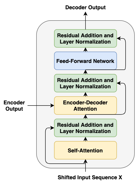
Decoders

Like the encoder, the Transformer architecture has six identical decoders stacked on top of each other. The following diagram shows the architecture of one of these stacked decoders. In addition to the self-attention and feedforward neural network present in the encoder, the decoder has an additional attention layer, which allows it to pay attention to the relevant parts in the output of the encoder stack.

The self-attention layer in the decoder is modified to allow positions to only attend to previous positions and not attend to subsequent positions. This is referred to as masked attention. Also, from the previous sections of this chapter, we remember that output embeddings are offset by 1 position in the decoder. This offsetting, along with the masked attention, ensures that while predicting for a particular position, we only have outputs from the previous positions available to us.

Like encoders, the output from each sub-layer here is applied with residual connects and layer normalization:

Now that we have understood the architecture for the Encoder and Decoder, let's look into the attention mechanism used in the Transformer architecture.

Self-attention

When trying to build a representation for a position in an input sequence, the self-attention mechanism allows the model to look at other positions/input tokens in the same sequence, which can help the model to build a better representation for this input position. This helps the model to infuse information about other tokens in the sequence that are relevant for a particular token when building the representation for this token.

Let's consider an example to understand this:

The man is eating a lot of mangoes and they seem to be his favorite fruit.

In this sentence, when the embedding of the word they is being built, the self-attention mechanism allows the representation of they to be highly influenced by the word mangoes and associates they with mangoes. Similarly, when the embedding for his is built, self-attention allows it to be associated with the word man.

How does self-attention work mathematically?

Self-attention tries to find the embedding of a token based on the other tokens in the sequence. For this purpose, it uses three abstractions, namely the key, query, and value vectors. Let's understand all of this now:

1. In the first step, the input embedding is multiplied by three matrices, Wk, Wq and Wv. This multiplication produces three embeddings, namely the key, query, and value embeddings. The model learns the three matrices, Wk, Wq, and Wv, during the training process as a result of backpropagation. The dimensionality of each of these embeddings is the same:

2. The second step is to understand how important the other tokens are for every individual token in the sequence. Let's say that we are computing the embedding for the second token. Our job is to figure out how important each token in the sequence is for the second token. This is found by performing the dot product between the query vector of the second token with the key vector of all tokens individually. This process can be thought of as the second token asking other tokens how important they are to it by sending the tokens its query vector, and the other tokens responding with their key vectors, and finally the dot product between them, giving the importance. Since the key and query vectors are of the same dimension, the output of this is a single number. Let's refer it as the score.

3. In the third step, the scores obtained for each word are divided by root , where d_k is the dimensionality of the key vector. In the standard Transformer, this is 64.

The softmax of the scores obtained from the previous step is performed next. This leads to stable gradients. The intuition here is that the higher the score for a token, the more important it is for the token whose representation is being computed.

4. Next, the value vector of each token is multiplied by its softmax score. As a result, the tokens that are more important for that position will have their values dominate the representation compared to tokens that are not that relevant for that specific position:

5. Finally, the obtained value vectors from the previous step are summed up to obtain the new representation for the token under consideration. The preceding diagram shows how the self-attention representation of the token Language is constructed for the input sequence Natural Language.

However, the Transformer doesn't just use a single attention head. The model uses multiple attention heads, which allows the model to focus on multiple different positions, instead of just one. The outputs from the multiple attention heads are concatenated and projected to provide the final values.

A small note on masked self-attention

Another important thing to understand is that inside the decoder, the multi-head attention mechanism is masked, meaning that it is only allowed to use representations from positions toward the left. This is because, while predicting the token for a particular position, only tokens from the left side would be available. As a result, all embeddings from the right are multiplied with 0 to mask them and the representations created can only be influenced by the tokens on the left.

Before we move on, let's quickly look into the encoder-decoder attention layer. This layer allows the decoder to capture contextual and positional information coming in from the encoder; basically, the information contained in the input sequence.

Now that we have discussed attention in detail, let's understand the rest of the components in the Transformer architecture shown in the following diagram:

Feedforward neural networks

Each encoder and decoder in the Transformer stack has a fully connected two-layer feedforward neural network with a ReLU activation function in between them. This feedforward neural network maps embeddings from one space to another space and the dimensionality of the inputs and outputs to these networks are the same.

Residuals and layer normalization

Residuals are applied to the output of each layer in a Transformer, thus enabling it to retain some information present in the previous layer. After the application of the residuals, the output is fed into layer normalization, which applies normalization across the features. The values calculated as a result are independent of the other examples.

Positional embeddings

Another interesting feature that we should try and capture is the sequential order of tokens in terms of the absolute position of the tokens, as well as features such as the relative distance between tokens. The Transformer architecture achieves this by using a positional embedding vector, which is added to the input embeddings. This model learns a pattern for this vector, which enables it to understand the aforementioned features.

How the decoder works

We have already seen the decoder's architecture and discussed the working of its internal components. Let's quickly try and throw light on the inputs to the decoder and the outputs from it. The output from the final encoder is transformed into a set of attention vectors represented by K and V. These outputs are received by the encoder-decoder attention layer in each of the decoders. Also, the decoder receives the embeddings for the tokens of the output sequence shifted by one, as happens in normal decoder operation. The decoder keeps producing outputs until it reaches the <end> token.

The linear layer and the softmax function

The decoder produces a vector of values as its output. Now, these values are projected to our vocabulary using the linear layer whose dimensionality is the same as the size of our vocabulary. The obtained values are normalized and a probability distribution is produced over the vocabulary using the softmax function, and the highest value is taken to be the output for that timestep. The index for the highest value is mapped to the vocabulary to obtain the predicted token.

The error computation happens in a similar way and the loss is backpropagated to the network for it to learn.

Transformer model summary

So, to summarize the architecture and training that we've looked at so far, the encoder receives an input embedding along with a position embedding, which are summed together and passed to a series of stacked encoders composed of self-attention and feedforward neural networks. The output from the last encoder is passed to the decoder, which itself contains the self-attention and feedforward neural network layers. In addition, the decoder contains an encoder-decoder attention layer, which helps it to understand the information coming in from the encoder. The decoder produces a vector as output, which is applied to a dense layer followed by softmax, and the word with the highest probability is taken as output for the given timestep. The error is computed based on the performance of the Transformer in predicting the output and the result is backpropagated for the network to learn.

BERT

The embeddings that we created when discussing Word2vec and fastText were static in the sense that no matter what context a word was being used in, its embedding would be the same.

Let's consider an example to understand this:

Apple is a fruit

Apple is a company

In both these sentences, no matter what context Apple is being used in, the embeddings for the word would be the same. Instead, we should work on building techniques that can provide representations of a word based on the current context it is being used in.

Moreover, we need to build semi-supervised models that could be pre-trained on a broader task and later be fine-tuned to a specific task. The knowledge built while solving the broader task could be applied to solve a different but related task. This is referred to as transfer learning.

BERT catered to both our aforementioned problems in its own unique way. Researchers at Google developed BERT and made the methodology that they used to build BERT open source, along with the pre-trained weights.

Let's look into the architecture for BERT next.

The BERT architecture

We read about Transformers in the previous section. BERT was built using the encoder component of the Transformer architecture. BERT is nothing but a set of stacked encoders, as we saw in the previous section. The researchers built two variants of the BERT model, as summarized in the following table:

The Transformer architecture upon which BERT was built had six stacked encoders. The hidden layer size (that is, the number of hidden units in the feedforward layers) was 512 and it had 8 self-attention heads. The details of the various layers in BERT are the same as what we discussed while talking about Transformers.

The BERT model input and output

Since the BERT model was built such that it could be fine-tuned to a wide variety of tasks, its inputs and outputs needed to be designed carefully such that they could handle single-sentence tasks such as text classification, along with two-sentence tasks such as question answering. The BERT model was built with a vocabulary of 30,000 words and used the WordPiece tokenizer for tokenization.

The BERT model input is explained in the following diagram. Let's try and understand each of the input components in the diagram.

The first input token to the BERT model is the [CLS] token, where CLS stands for Classification. It is a special token and the final hidden state output from the BERT model corresponding to this token is used for classification tasks. The [CLS] token carries the output for single-sentence classification tasks.

For two-sentence tasks, the sentences are brought in together and separated by a special [SEP] token, which helps to differentiate between the sentences. In addition to the [SEP] token, an additional learned embedding is added to the token to represent whether it belongs to the first sentence or the second.

As with Transformers, a positional embedding is added to the tokens for the same reason we discussed regarding Transformers.

Hence, the input for every token to the BERT model is a sum of the token embeddings, positional embeddings, and segment embeddings:

Now that we have talked about the inputs, let's briefly discuss the outputs. The BERT model at every position on a vector of size 768 is BERT_BASE and a vector of size 1024 is the BERT_LARGE model. These output vectors can be used differently depending on the fine-tuning task to be solved.

So, we've understood that BERT is such a cool thing, along with its architecture and the inputs and outputs for the model. One thing that we haven't got a sense of yet is how it was trained. Let's investigate this now.

How did BERT the pre-training happen?

The BERT model was pre-trained using two unsupervised tasks, namely the masked language model and next-sentence prediction. Let's look at the details of these next.

The masked language model

Conditional language models prior to BERT were built using either the left-to-right approach or the right-to-left approach. We know that a bidirectional approach that can look both backward and forward would be more powerful than a unidirectional model. However, since with Transformers we have a multilayered context, the bidirectional approach would allow each token to indirectly see itself.

How do we build a model that can be conditioned using both the left and right contexts?

The developers of BERT decided to use masks to allow bidirectional conditioning. The BERT model picks 15% of the tokens at random and masks them. Next, it tries to predict these masked tokens. This process is referred to as Masked Language Modeling (MLM).

However, there is a problem with this approach: the [MASK] token will not be present during fine-tuning. In order to resolve this, among the 15% of the tokens chosen at random, let's say if the ith token is chosen, then the following would happen:

• It would be replaced with the [MASK] token 80% of the time (80% of 15% = 125 of the times).
• It will be replaced with a random token 10% of the time (10% of 15% = 1.5% of the time).
• It is kept unchanged for the remaining 10% of the time (10% of 15% = 1.5% of the time).

Next-sentence prediction

During the MLM task, we did not really work with multiple sentences. However, with BERT, the thought process was to accommodate the possibility of tasks involving a pair of sentences, as often happens in question answering tasks, where the relationships between multiple sentences need to be captured. In order to do this, BERT resorted to working with a next-sentence prediction task. A pair of sentences, A and B, are input to the model such that 50% of the time, sentence B would actually be the next sentence in the corpus after sentence A where the labeling used would be IsNext, and it would not be the next sentence 50% of the time, where the labeling would be NotNext. In the next-sentence prediction task, the model would be asked to predict whether sentence B is actually the next sentence following sentence A or not.

Now we know how the BERT pre-training worked, let's look into the fine-tuning of BERT next and understand how its outputs can be utilized.

For the purpose of pre-training, we used as our datasets the Book Corpus, comprising 800 million words, and English Wikipedia, comprising 2.5 billion words.

BERT fine-tuning

The pre-trained weights developed using the ways we've discussed can now be fine-tuned to cater to a number of tasks. Let's look at those next.

For single classification tasks, the output for position 1 carries information about the classification label. The vector from the first position is sent across to a feedforward neural network, followed by the application of the softmax function, which returns the probability distribution for the number of classes involved in the task, as shown in the following diagram:

Similarly, for sentence-pair text classification tasks, such as whether the second sentence follows the first sentence in a corpus or the second sentence is the answer to the first sentence (a question), these are classification tasks where we need to respond with a Yes or No answer. Such tasks can also make use of the first output vector to determine the results, as shown in the following diagram:

Named Entity Recognition (NER)-like tasks want an output for each input token. For example, in an NER task, we may require the model to figure out whether the tokens in a sentence refer to a person, location, date, and so on. Each token must say which entity it is catering to from the ones we've mentioned. This is a Seq2Seq task where the size of the input should be equal to the size of the output. The BERT model outputs a vector for each position. Now, each of these position outputs can be fed to a neural network to figure out the named entity for a particular token. This is illustrated in the following diagram:

Similarly, the BERT model can be fine-tuned for other tasks such as question answering, as shown in the following diagram:

Ideas for these have been sourced original BERT paper, BERT: Pre-Training of Deep Bidirectional Transformers for Language Understanding by Delvin et al., available at https://arxiv.org/pdf/1810.04805.pdf.

The rise of BERT revolutionized the domain of NLP and great improvements were achieved in solving numerous tasks. BERT even outperformed all the previous benchmark results for certain tasks.

The open source code for BERT is available on GitHub at https://github.com/google-research/bert.

An approach to fine-tune the BERT model for the question classification task we tried solving in Chapter 8, From Human Neurons to Artificial Neurons for Text Understanding, was made, and the code has been posted at https://github.com/amankedia/Question-Classification-using-BERT, along with the results.

Similarly, BERT can be applied to numerous tasks such as part-of-speech tagging, building chatbots, and so on.

Summary

In this chapter, we had a look at some of the recent advancements in the field of NLP, encompassing Seq2Seq modeling, the attention mechanism, the Transformer model, and BERT, all of which have revolutionized the way NLP problems are approached today. We began with a discussion on Seq2Seq modeling where we looked at its core components, the encoder and decoder. Based on the knowledge garnered, we built a French-to-English translator using the encoder-decoder stack. After that, we had a detailed discussion on the attention mechanism, which has allowed great parallelization leading to fast NLP training, and has also improved upon the results from the existing architectures. Next, we looked at Transformers and discussed every component inside the encoder-decoder stack of the Transformers. We also saw how the attention mechanism can be used as the core building block of such architectures, and can possibly provide a replacement for the existing RNN-based architectures. Finally, we had an in-depth discussion on BERT, which is a very recent development that has paved the way for building highly efficient, fine-tuned NLP models for a wide variety of tasks.

Throughout this book, attempts were made to understand multiple NLP techniques and how they could be applied to solve a plethora of problems related to NLP. We built numerous applications such as a chatbot, a spell-checker, a sentiment analyzer, a question classifier, a sarcasm detector, a language generator, and a language translator, among many others throughout the course of this book. As a result, along with the theoretical knowledge we've acquired, we've had plenty of necessary hands-on experience in solving NLP problems as well.