Natural Language Processing (NLP) research and development is occurring concurrently in many programming languages. Some very popular NLP libraries are written in various programming languages, such as Java, Python, and C++. However, we have chosen to write this book in Python and, in this chapter, we'll discuss the merits of using Python to delve into NLP. We'll also introduce the important Python libraries and tools that we will be using throughout this book.
In the chapter, we'll cover the following topics:
- Understanding Python with NLP
- Important Python libraries
- Web scraping libraries and methodology
- Overview of Jupyter Notebook
Let's get started!
Technical requirements
The code files for this chapter can be found at the following GitHub link: https://github.com/PacktPublishing/Hands-On-Python-Natural-Language-Processing/tree/master/Chapter02.
Understanding Python with NLP
Python is a high-level, object-oriented programming language that has experienced a meteoric rise in popularity. It is an open source programming language, meaning anyone with a functioning computer can download and start using Python. Python's syntax is simple and aids in code readability, ease of use in terms of debugging, and supports Python modules, thereby encouraging modularity and scalability.
In addition, it has many other features that contribute to its halo and make it an extremely popular language in the developer community. A prominent drawback often attributed to Python is its relatively slower execution speed compared to compiled languages. However, Python's performance is shown to be comparable to other languages and it can be vastly improved by employing clever programming techniques or using libraries built using compiled languages.
If you are a Python beginner, you may consider downloading the Python Anaconda distribution (https://www.anaconda.com/products/individual), which is a free and open source distribution for scientific computing and data science. Anaconda has a number of very useful libraries and it allows very convenient package management (installing/uninstalling applications). It also ships with multiple Interactive Development Environments (IDEs) such as Spyder and Jupyter Notebook, which are some of the most widely used IDEs due to their versatility and ease of use. Once downloaded, the Anaconda suite can be installed easily. You can refer to the installation documentation for this (https://docs.anaconda.com/anaconda/install/).
After installing Anaconda, you can use the Anaconda Prompt (this is similar to Command Prompt, but it lets you run Anaconda commands) to install any Python library using any of the Anaconda's package managers. pip and conda are the two most popular package managers and you can use either to install libraries.
The following is a screenshot of the Anaconda Prompt with the command to install the pandas library using pip:

Now that we know how to install libraries, let's explore the simplicity of Python in terms of carrying out reasonably complex tasks.
We have a CSV file with flight arrival and departure data from major US airports from July 2019. The data has been sourced from the US Department of Transportation website (https://www.transtats.bts.gov/DL_SelectFields.asp?Table_ID=236).
The file extends to more than half a million rows. The following is a partial snapshot of the dataset:
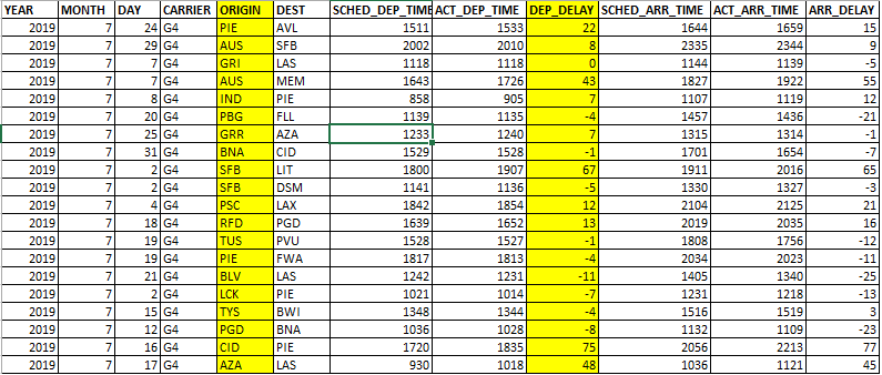
We are interested to know about which airport has the longest average delay in terms of flight departure. This task was completed using the following three lines of code. The pandas library can be installed using pip, as discussed previously:
import pandas as pd

data = pd.read_csv("flight_data.csv")
data.groupby("ORIGIN").mean()["DEP_DELAY"].idxmax()
Here's the output:
Out[15]: 'PPG'
So, it turns out that a remote airport (Pago Pago international airport) somewhere in the American Samoa had the longest average departure delays recorded in July 2019. As you can see, a relatively complex task was completed using only three lines of code. The simple-looking, almost English-like code helped us read a large dataset and perform quantitative analysis in a fraction of a second. This sample code also showcases the power of Python's modular programming.
In the first line of the code, we imported the pandas library, which is one of the most important libraries of the Python data science stack. Please refer pandas' documentation page (https://pandas.pydata.org/docs/) for more information, which is quite helpful and easy to follow. By importing the pandas library, we were able to avoid writing the code for reading a CSV file line by line and parsing the data. It also helped us utilize pre-coded pandas functions such as idxmax(), which returns the index of the maximum value of a row or column in a data frame (a pandas object that stores data in tabular format). Using these functions significantly reduced our effort in getting the required information.
Other programming languages have powerful libraries too, but the difference is that Python libraries tend to be very easy to install, import, and deploy. In addition, the large, open source developer community of Python translates to a vast number of very useful libraries being made available regularly. It's no surprise, then, that Python is particularly popular in the data science and machine learning domain and that the most widely used Machine Learning (ML) and DS libraries are either Python-based or are Python wrappers. Since NLP draws a lot from data science, ML, and Deep Learning (DL) disciplines, Python is very much becoming the lingua franca for NLP as well.
Python's utility in NLP
Learning a new language is not easy. For an average person, it can take months or even years to attain intermediate level fluency in a new language. It requires an understanding of the language's syntax (grammar), memorizing its vocabulary, and so on, to gain confidence in that language. Likewise, it is also quite challenging for computers to learn natural language since it is impractical to code every single rule of that language.
Let's assume we want to build a virtual assistant that reads queries submitted by a website's users and then directs them to the appropriate section of the website. Let's say the virtual assistant receives a request stating, How do we change the payment method and payment frequency?
If we want to train our virtual assistant the human way, then we will need to upload an English dictionary in its memory (the easy part), find a way to teach it English grammar (speech, clause, sentence structure, and so on), and logical interpretation. Needless to say, this approach is going to require a herculean effort. However, what if we could transform the sentence into mathematical objects so that the computer can apply mathematical or logical operations and make some sense out of it? That mathematical construct can be a vector, matrix, and so on.
For example, what if we assume an N-dimensional space where each dimension (axis) of the space corresponds to a word from the English vocabulary? With this, we can represent the preceding statement as a vector in that space, with its coordinate along each axis being the count of the word representing that axis. So, in the given sentence, the sentence vector's magnitude along the payment axes will be 2, the frequency axes will be 1, and so on. The following is some sample code we can use to achieve this vectorization in Python. We will use the scikit-learn library to perform vectorization, which can be installed by running the following command in the Anaconda Prompt:
pip install scikit-learn
Using the CountVectorizer module of Python's scikit-learn library, we have vectorized the preceding sentence and generated the output matrix with the vector (we will go into the details of this in subsequent chapters):
from sklearn.feature_extraction.text import CountVectorizer

sentence = ["How to change payment method and payment frequency"]
vectorizer = CountVectorizer(stop_words='english')
vectorizer.fit_transform(sentence).todense()
Here is the output:
matrix([[1, 1, 1, 2]]), dtype=int64)
This vector can now be compared with other sentence vectors in the same N-dimensional space and we can derive some sort of meaning or relationship between these sentences by applying vector principles and properties. This is an example of how a sentence comprehension task could be transformed into a linear algebra problem. However, as you may have already noticed, this approach is computationally intensive as we need to transform sentences into vectors, apply vector principles, and perform calculations. While this approach may not yield a perfectly accurate outcome, it opens an avenue for us to explore by leveraging mathematical theorems and established bodies of research.
Expecting humans to use this approach for sentence comprehension may be impractical, but computers can do these tasks fairly easily, and that's where programming languages such as Python become very useful in NLP research. Please note that the example in this section is just one example of transforming an NLP problem into a mathematical construct in order to facilitate processing. There are many other methods that will be discussed in detail in this book.
Important Python libraries
We will now discuss some of the most important Python libraries for NLP. We will delve deeper into some of these libraries in subsequent chapters.
NLTK
The Natural Language Toolkit library (NLTK) is one of the most popular Python libraries for natural language processing. It was developed by Steven Bird and Edward Loper of the University of Pennsylvania. Developed by academics and researchers, this library is intended to support research in NLP and comes with a suite of pedagogical resources that provide us with an excellent way to learn NLP. We will be using NLTK throughout this book, but first, let's explore some of the features of NLTK.
However, before we do anything, we need toinstall the library by running the following command in the Anaconda Prompt:
pip install nltk
NLTK corpora
A corpus is a large body of text or linguistic data and is very important in NLP research for application development and testing. NLTK allows users to access over 50 corpora and lexical resources (many of them mapped to ML-based applications). We can import any of the available corpora into our program and use NLTK functions to analyze the text in the imported corpus. More details about each corpus could be found here: http://www.nltk.org/book/ch02.html
Text processing
As discussed previously, a key part of NLP is transforming text into mathematical objects. NLTK provides various functions that help us transform the text into vectors. The most basic NLTK function for this purpose is tokenization, which splits a document into a list of units. These units could be words, alphabets, or sentences.
Refer to the following code snippet to perform tokenization using the NLTK library:
import nltk

text = "Who would have thought that computer programs would be analyzing human sentiments"

from nltk.tokenize import word_tokenize

tokens = word_tokenize(text)
print(tokens)
Here's the output:
['Who', 'would', 'have', 'thought', 'that', 'computer', 'programs', 'would', 'be', 'analyzing', 'human', 'sentiments']
We have tokenized the preceding sentence using the word_tokenize() function of NLTK, which is simply splitting the sentence by white space. The output is a list, which is the first step toward vectorization.
In our earlier discussion, we touched upon the computationally intensive nature of the vectorization approach due to the sheer size of the vectors. More words in a vector mean more dimensions that we need to work with. Therefore, we should strive to rationalize our vectors, and we can do that using some of the other useful NLTK functions such as stopwords, lemmatization, and stemming.
The following is a partial list of English stop words in NLTK. Stop words are mostly connector words that do not contribute much to the meaning of the sentence:
import nltk

stopwords = nltk.corpus.stopwords.words('english')
print(stopwords)
Here's the output:
['i', 'me', 'my', 'myself', 'we', 'our', 'ours', 'ourselves', 'you', "you're", "you've", "you'll", "you'd", 'your', 'yours', 'yourself', 'yourselves', 'he', 'him', 'his', 'himself', 'she', "she's", 'her', 'hers', 'herself', 'it', "it's", 'its', 'itself', 'they', 'them', 'their', 'theirs', 'themselves', 'what', 'which', 'who', 'whom', 'this', 'that', "that'll", 'these', 'those', 'am', 'is', 'are', 'was', 'were', 'be', 'been', 'being', 'have', 'has', 'had', 'having', 'do', 'does', 'did', 'doing', 'a', 'an', 'the', 'and', 'but', 'if', 'or', 'because', 'as', 'until', 'while', 'of', 'at', 'by', 'for', 'with', 'about', 'against', 'between', 'into', 'through', 'during', 'before', 'after', 'above', 'below', 'to', 'from', 'up', 'down', 'in', 'out', 'on', 'off', 'over', 'under', 'again', 'further', 'then', 'once', 'here', 'there', 'when', 'where', 'why', 'how', 'all', 'any', 'both', 'each', 'few', 'more', 'most', 'other', 'some', 'such', 'no', 'nor', 'not', 'only', 'own', 'same', 'so', 'than', 'too', 'very', 's', 't', 'can', 'will', 'just', 'don', "don't", 'should', "should've", 'now', 'd', 'll', 'm', 'o', 're', 've', 'y', 'ain', 'aren', "aren't", 'couldn', "couldn't", 'didn', "didn't", 'doesn', "doesn't", 'hadn', "hadn't", 'hasn', "hasn't", 'haven', "haven't", 'isn', "isn't", 'ma', 'mightn', "mightn't", 'mustn', "mustn't", 'needn', "needn't", 'shan', "shan't", 'shouldn', "shouldn't", 'wasn', "wasn't", 'weren', "weren't", 'won', "won't", 'wouldn', "wouldn't"]
Since NLTK provides us with a list of stop words, we can simply look up this list and filter out stop words from our word list:
newtokens=[word for word in tokens if word not in stopwords]
Here's the output:
['Who',
 'would',
 'thought',
 'computer',
 'programs',
 'would',
 'analyzing',
 'human',
 'sentiments']
We can further modify our vector by using lemmatization and stemming, which are techniques that are used to reduce words to their root form. The rationale behind this step is that the imaginary n-dimensional space that we are navigating doesn't need to have separate axes for a word and that word's inflected form (for example, eat and eating don't need to be two separate axes). Therefore, we should reduce each word's inflected form to its root form. However, this approach has its critics because, in many cases, inflected word forms give a different meaning than the root word. For example, the sentences My manager promised me promotion and He is a promising prospect use the inflected form of the root word promise but in entirely different contexts. Therefore, you must perform stemming and lemmatization after considering its pros and cons.
The following code snippet shows an example of performing lemmatization using the NLTK library's WordNetlemmatizer module:
from nltk.stem import WordNetLemmatizer

text = "Who would have thought that computer programs would be analyzing human sentiments"
tokens = word_tokenize(text)
lemmatizer = WordNetLemmatizer()
tokens=[lemmatizer.lemmatize(word) for word in tokens]
print(tokens)
Here's the output:
['Who', 'would', 'have', 'thought', 'that', 'computer', 'program', 'would', 'be', 'analyzing', 'human', 'sentiment']
Lemmatization is performed by looking up a word in WordNet's inbuilt root word map. If the word is not found, it returns the input word unchanged. However, we can see that the performance of the lemmatizer was not good and it was only able to reduce programs and sentiments from their plural forms. This shows that the lemmatizer is highly dependent on the root word mapping and is highly susceptible to incorrect root word transformation.
Stemming is similar to lemmatization but instead of looking up root words in a pre-built dictionary, it defines some rules based on which words are reduced to their root form. For example, it has a rule that states that any word with ing as a suffix will be reduced by removing the suffix.
The following code snippet shows an example of performing stemming using the NLTK library's PorterStemmer module:
from nltk.stem import PorterStemmer
from nltk.tokenize import word_tokenize

text = "Who would have thought that computer programs would be analyzing human sentiments"
tokens=word_tokenize(text.lower())
ps = PorterStemmer()
tokens=[ps.stem(word) for word in tokens]
print(tokens)
Here's the output:
['who', 'would', 'have', 'thought', 'that', 'comput', 'program', 'would', 'be', 'analyz', 'human', 'sentiment']
As per the preceding output, stemming was able to transform more words than lemmatizing, but even this is far from perfect. In addition, you will notice that some stemmed words are not even English words. For example, analyz was derived from analyzing as it blindly applied the rule of removing ing.
The preceding examples show the challenges of reducing words correctly to their respective root forms using NLTK tools. Nevertheless, these techniques are quite popular for text preprocessing and vectorization. You can also create more sophisticated solutions by building on these basic functions to create your own lemmatizer and stemmer. In addition to these tools, NLTK has other features that are used for preprocessing, all of which we will discuss in subsequent chapters.
Part of speech tagging
Part of speech tagging (POS tagging) identifies the part of speech (noun, verb, adverb, and so on) of each word in a sentence. It is a crucial step for many NLP applications since, by identifying the POS of a word, we can deduce its contextual meaning. For example, the meaning of the word ground is different when it is used as a noun; for example, The ground was sodden due to rain, compared to when it is used as an adjective, for example, The restaurant's ground meat recipe is quite popular. We will get into the details of POS tagging and its applications, such as Named Entity Recognizer (NER), in subsequent chapters.
Refer to the following code snippets to perform POS tagging using NLTK:
nltk.pos_tag(["your"])
Out[148]: [('your', 'PRP$')]

nltk.pos_tag(["beautiful"])
Out[149]: [('beautiful', 'NN')]

nltk.pos_tag(["eat"])
Out[150]: [('eat', 'NN')]
We can pass a word as a list to the pos_tag() function, which outputs the word and its part of speech. We can generate POS for each word of a sentence by iterating over the token list and applying the pos_tag() function individually. The following code is an example of how POS tagging can be done iteratively:
from nltk.tokenize import word_tokenize
text = "Usain Bolt is the fastest runner in the world"
tokens = word_tokenize(text)
[nltk.pos_tag([word]) for word in tokens]
Here's the output:
[[('Usain', 'NN')],
 [('Bolt', 'NN')],
 [('is', 'VBZ')],
 [('the', 'DT')],
 [('fastest', 'JJS')],
 [('runner', 'NN')],
 [('in', 'IN')],
 [('the', 'DT')],
 [('world', 'NN')]]
The exhaustive list of NLTK POS tags can be accessed using the upenn_tagset() function of NLTK:
import nltk

nltk.download('tagsets') # need to download first time
nltk.help.upenn_tagset()
Here is a partial screenshot of the output:

Textblob
Textblob is a popular library used for sentiment analysis, part of speech tagging, translation, and so on. It is built on top of other libraries, including NLTK, and provides a very easy-to-use interface, making it a must-have for NLP beginners. In this section, we would like you to dip your toes into this very easy-to-use, yet very versatile library. You can refer to Textblob's documentation, https://textblob.readthedocs.io/en/dev/, or visit its GitHub page, https://github.com/sloria/TextBlob, to get started with this library.
Sentiment analysis
Sentiment analysis is an important area of research within NLP that aims to analyze text and assess its sentiment. The Textblob library allows users to analyze the sentiment of a given piece of text in a very convenient way. Textblob library's documentation (https://textblob.readthedocs.io/en/dev/) is quite detailed, easy to read, and contains tutorials as well.
We can install the textblob library and download the associated corpora by running the following commands in the Anaconda Prompt:
pip install -U textblob
python -m textblob.download_corpora
Refer to the following code snippet to see how conveniently the library can be used to calculate sentiment:
from textblob import TextBlob

TextBlob("I love pizza").sentiment
Here's the output:
Sentiment(polarity=0.5, subjectivity=0.6)
Once the TextBlob library has been imported, all we need to do to calculate the sentiment is to pass the text that needs to be analyzed and use the sentiment module of the library. The sentiment module outputs a tuple with the polarity score and subjectivity score. The polarity score ranges from -1 to 1, with -1 being the most negative sentiment and 1 being the most positive statement. The subjectivity score ranges from 0 to 1, with a score of 0 implying that the statement is factual, whereas a score of 1 implies a highly subjective statement.
For the preceding statement, I love pizza, we get a polarity score of 0.5, implying a positive sentiment. The subjectivity of the preceding statement is also calculated as high, which seems correct. Let's analyze the sentiment of other sentences using Textblob:
TextBlob("The weather is excellent").sentiment
Here's the output:
Sentiment(polarity=1.0, subjectivity=1.0)
The polarity of the preceding statement was calculated as 1 due to the word excellent.
Now, let's look at an example of a highly negative statement. Here, the polarity score of -1 is due to the word terrible:
TextBlob("What a terrible thing to say").sentiment
Here's the output:
Sentiment(polarity=-1.0, subjectivity=1.0)
It also appears that polarity and subjectivity have a high correlation.
Machine translation
Textblob uses Google Translator's API to provide a very simple interface for translating text. Simply use the translate() function to translate a given text into the desired language (from Google's catalog of languages). The to parameter in the translate() function determines the language that the text will be translated into. The output of the translate() function will be the same as what you will get in Google Translate.
Here, we have translated a piece of text into three languages (French, Mandarin, and Hindi). The list of language codes can be obtained from https://cloud.google.com/translate/docs/basic/translating-text#language-params:
from textblob import TextBlob

languages = ['fr','zh-CN','hi']
for language in languages:
    print(TextBlob("Who knew translation could be fun").translate(to=language))
Here's the output:

Part of speech tagging
Textblob's POS tagging functionality is built on top of NLTK's tagging function, but with some modifications. You can refer to NLTK's documentation on POS tagging for more details: https://www.nltk.org/book/ch05.html
The tags function performs POS tagging like so:
TextBlob("The global economy is expected to grow this year").tags
Here's the output:
[('The', 'DT'),
 ('global', 'JJ'),
 ('economy', 'NN'),
 ('is', 'VBZ'),
 ('expected', 'VBN'),
 ('to', 'TO'),
 ('grow', 'VB'),
 ('this', 'DT'),
 ('year', 'NN')]
Since Textblob uses NLTK for POS tagging, the POS tags are the same as NLTK. This list can be accessed using the upenn_tagset() function of NLTK:
import nltk

nltk.download('tagsets') # need to download first time
nltk.help.upenn_tagset()
These are just a few popular applications of Textblob and they demonstrate the ease of use and versatility of the program. There are many other applications of Textblob, and you are encouraged to explore them. A good place to start your Textblob journey and familiarize yourself with other Textblob applications would be the Textblob tutorial, which can be accessed at https://textblob.readthedocs.io/en/dev/quickstart.html.
VADER
Valence Aware Dictionary and sEntiment Reasoner (VADER) is a recently developed lexicon-based sentiment analysis tool whose accuracy is shown to be much greater than the existing lexicon-based sentiment analyzers. This model was developed by computer science professors from Georgia Tech and they have published the methodology of building the lexicon in their very easy-to-read paper (http://comp.social.gatech.edu/papers/icwsm14.vader.hutto.pdf). It improves on other sentiment analyzers by including colloquial language terms, emoticons, slang, acronyms, and so on, which are used generously in social media. It also factors in the intensity of words rather than classifying them as simply positive or negative.
We can install VADER by running the following command in the Anaconda Prompt:
pip install vaderSentiment
The following is an example of VADER in action:
from vaderSentiment.vaderSentiment import SentimentIntensityAnalyzer
analyser = SentimentIntensityAnalyzer()
First, we need to import SentimentIntensityAnalyzer module from the vaderSentiment library and create an analyser object of the SentimentIntensityAnalyzer class. We can now pass any text into this object and it will return the sentiment analysis score. Refer to the following example:
analyser.polarity_scores("This book is very good")
Here's the output:
{'neg': 0.0, 'neu': 0.556, 'pos': 0.444, 'compound': 0.4927}
Here, we can see that VADER outputs the negative score, neutral score, and positive score and then aggregates them to calculate the compound score. The compound score is what we are interested in. Any score greater than 0.05 is considered positive, while less than -0.05 is considered negative:
analyser.polarity_scores("OMG! The book is so cool")
Here's the output:
{'neg': 0.0, 'neu': 0.604, 'pos': 0.396, 'compound': 0.5079}
While analyzing the preceding sentence, VADER correctly interpreted the colloquial terms (OMG and cool) and was able to quantify the excitement of the statement. The compound score is greater than the previous statement, which seems reasonable.
Web scraping libraries and methodology
While discussing NLTK, we highlighted the significance of a corpus or large repository of text for NLP research. While the available corpora are quite useful, NLP researchers may require the text of a particular subject. For example, someone trying to build a sentiment analyzer for financial markets may not find the available corpus (presidential speeches, movie reviews, and so on) particularly useful. Consequently, NLP researchers may have to get data from other sources. Web scraping is an extremely useful tool in this regard as it lets users retrieve information from web sources programmatically.
Before we start discussing web scraping, we wish to underscore the importance of complying with the respective website policies on web scraping. Most websites allow web scraping for individual non-commercial use, but you must always confirm the policy before scraping a website.
To perform web scraping, we will be using a test website (https://webscraper.io/test-sites/e-commerce/allinone) to implement our web scraping script. The test website is that of a fictitious e-commerce company that sells computers and phones.
Here's a screenshot of the website:

The website lists the products that it sells and each product has price and user rating information. Let's say we want to extract the price and user ratings of every laptop listed on the website. You can do this task manually, but that would be very time-consuming and inefficient. Web scraping helps us perform tasks like this much more efficiently and elegantly.
Now, let's get into how the preceding task could be carried out using web scraping tools in Python. First, we need to install the Requests and BeautifulSoup libraries, which are the most commonly used Python libraries for web scraping. The documentation for Requests can be accessed at https://requests.readthedocs.io/en/master/, while the documentation for BeatifulSoup can be accessed at https://www.crummy.com/software/BeautifulSoup/:
          pip install requests


          pip install beautifulsoup4
Once installed, we will import the Requests and BeautifulSouplibraries. The pandas library will be used to store all the extracted data in a data frame and export data into a CSV file:
import requests
from bs4 import BeautifulSoup
import pandas as pd
When we type a URL into our web browser and hit Enter, a set of events get triggered before the web page gets rendered in our browser. These events include our browser looking up the IP address of the website, our browser sending an HTTP request to the server hosting the website, and the server responding by sending another HTTP response. If everything is agreed to, a handshake between the server and your browser occurs and the data is transferred. The request library helps us perform all these steps using Python scripts.
The following code snippet shows how we can programmatically connect to the website using the Requests library:
url = 'https://webscraper.io/test-sites/e-commerce/allinone/computers/laptops'
request = requests.get(url)
Running the preceding commands establishes a connection with the given website and reads the HTML code of the page. Everything we see on a website (text, images, layouts, links to other web pages, and so on) can be found in the HTML code of the page. Using the .text function of request, we can output the entire HTML script of the web page, as shown here:
request.text
Here's the output:

If you want to see the HTML code of the page on your browser, simply right-click anywhere on the page and select Inspect, as shown here:

This will open a panel containing the HTML code of the page. If you hover your mouse over any part of the HTML code, the corresponding section on the web page will be highlighted. This tells us that the code for the highlighted portion of the web page's code can be found by expanding that section of the HTML code:

HTML code is generally divided into sections, with a typical page having a header section and a body section. The body section is further divided into elements, with each element having attributes that are represented by a specific tag. In the preceding screenshot, we can see the various elements, classes, and tags of the HTML code. We will need to navigate through this complex-looking code and extract the relevant information (in our case, the product title, price, and rating). This seemingly complex task can be carried out quite conveniently using any of the web scraping libraries available. Beautiful Soup is one of the most popular scrapers out there, so we will see how it can help us parse the intimidating HTML code text. We strongly encourage you to visit Beautiful Soup's documentation page (https://www.crummy.com/software/BeautifulSoup/bs4/doc/) and gain a better understanding of this fascinating library.
We use the BeautifulSoup module and pass the HTML code (request.text) and a parameter called HTML Parser to it, which creates a BeautifulSoup HTML parser object. We can now apply many of the versatile BeautifulSoup functions to this object and extract the information that we seek. But before we start doing that, we will have to familiarize ourselves with the web page we are trying to scrape and identify where on the web page the elements that we are interested in are to be found. In the e-commerce website's HTML code, we can see that each product's detail is coded within a <div> tag (div refers to division in HTML) with col-sm-4 col-lg-4 col-md-4 as the class. If you expand the <div> tag by clicking on the arrow, you will see that, within the <div> tag, there are other tags and elements as well that store various pieces of information.
To begin with, we are interested in getting the list of product names. To find out where in the HTML code the product names are incorporated, we will have to hover the cursor above any of the product's names, right-click, and then click on Inspect.
This will open a panel containing the web page's HTML code, as shown in the following screenshot:
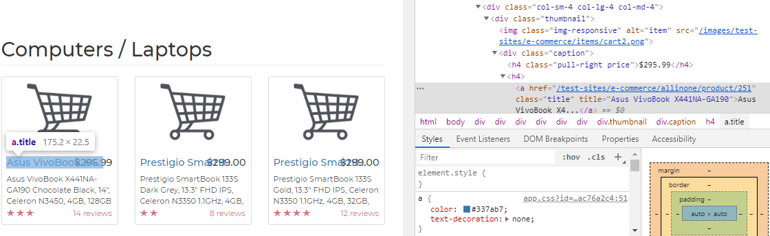
As we can see, the name of the product can be extracted from the title element of the <a> tag, which is within the caption subdivision of the code. Likewise, we can also find price information within the same caption subdivision but under the pull-right price class. Lastly, rating information can be extracted from the subdivision with the rating class:

We can now start formulating our web scraping strategy, which will involve iterating over all the code divisions with the col-sm-4 col-lg-4 col-md-4 class and then extracting the relevant information in each iteration. We'll use Beautiful Soup's find_all() function to identify all the <div> tags of the col-sm-4 col-lg-4 col-md-4 class. This function creates an iteratable object and we use a for loop to search each subdivision. We can extract the text from a BeautifulSoup object by using the .text function and can extract the name of an element by using the .get() function. Please refer to the following scraping code:
titles = []
prices = []
ratings = []
url = 'https://webscraper.io/test-sites/e-commerce/allinone/computers/laptops'
request = requests.get(url)
soup = BeautifulSoup(request.text, "html.parser")
for product in soup.find_all('div', {'class': 'col-sm-4 col-lg-4 col-md-4'}):
    for pr in product.find_all('div', {'class': 'caption'}):
        for p in pr.find_all('h4', {'class': 'pull-right price'}):
            prices.append(p.text)
        for title in pr.find_all('a' , {'title'}):
            titles.append(title.get('title'))
    for rt in product.find_all('div', {'class': 'ratings'}):
        ratings.append(len(rt.find_all('span',
                      {'class': 'glyphicon glyphicon-star'})))
As the last step, we pass the extracted information to a data frame and export the final result in a CSV file or other file type:
product_df = pd.data frame(zip(titles,prices,ratings), columns =
                            ['Titles','Prices', 'Ratings'])

product_df.to_csv("ecommerce.csv",index=False)
The following is a partial screenshot of the file that was created:

Likewise, you can extract text information, such as user reviews and product descriptions, for NLP-related projects. Please note that scraped data may require further processing based on requirements.
The preceding steps demonstrate how we can programmatically extract relevant information from web sources using web scraping with relative ease using applicable Python libraries. The more complex the structure of a web page is, the more difficult it is to scrape that page. Websites also keep changing the structure and format of their web pages, which means large-scale changes need to be made to the underlying HTML code. Any change in the HTML code of the page necessitates a review of your scraping code. You are encouraged to practice scraping other websites and gain a better understanding of HTML code structure. We would like to reiterate that it is imperative that you comply with any web scraping restrictions or limits put in place by that website.
Overview of Jupyter Notebook
IDEs are software applications that provide software programmers with a suite of services such as coding interfaces, debugging, and compiling/interpreting. Python programmers are spoilt for choice as there are many open source IDEs for Python, including Jupyter Notebook, spyder, atom, and pycharm, and each IDE comes with its own set of features. We have used Jupyter Notebook for this book. and all the code and exercises discussed in this book can be accessed at https://github.com/PacktPublishing/Hands-On-Python-Natural-Language-Processing.
Jupyter Notebook is the IDE of choice for pedagogical purposes as it allows us to weave together code blocks, narrative, multimedia, and graphs in one flowing notebook format. It comes pre-packaged with the Anaconda Python distribution and installing it is quite simple. Please refer to the very nicely written beginner's guide, which should help you gain a basic understanding of Jupyter Notebook: https://jupyter-notebook-beginner-guide.readthedocs.io/en/latest/execute.html.
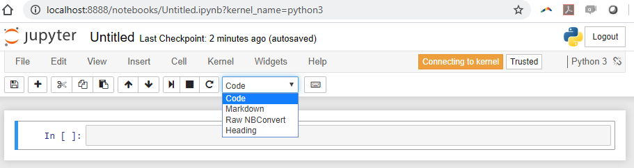
Jupyter Notebook has an .ipynb extension. In order to launch a notebook, open the terminal (if you have installed Anaconda, please use the Anaconda Prompt) and cd to the directory where the notebook is located. Run the jupyter notebook command, which will launch a starter page that lists the files stored in that location. You can either select an existing notebook to open or create a new notebook by clicking on the New button and selecting Python3, as shown in the following screenshot:

This will create a new notebook with a single cell. By default, this cell is meant for you to type your code into it. However, using the drop-down menu shown in the following screenshot, you can toggle between Code and Markdown (text):
You can either use the icons in the notebook to insert/run cells or use hot keys such as Shift + Enter to run the current cell, Ctrl + Enter to run multiple selected cells, A to insert a cell above, B to insert a cell below, and so on. Once you have completed working on the notebook, you can save it in the format of your choice by navigating to File | Download as, as shown in the following screenshot. Jupyter provides various options for you to save the file based on the requirement (although you would typically want to save it in Jupyter Notebook (.ipynb) format):

You can also access a finished notebook (a pre-existing .ipynb file) by running the jupyter notebook <filename> command. This will open the required notebook in a browser. The following are some screenshots of launching and working on a completed notebook.
The following is a screenshot of running a Jupyter Notebook cell with code:

The following screenshot shows how variables can be visualized in Jupyter Notebook inline by running the variable name. You can also see how bar plots can be rendered inline by running the barplot command:

The following screenshot shows how easily you can render a histogram or distribution plot in the Jupyter notebook and how you can add text just below the plot to explain the main points to potential readers:

The following screenshot shows how a count plot can be rendered inline and explained using rich text:

Given its powerful features and ease of use, Jupyter Notebook has become one of the most popular Python IDEs in both academia and industries. Please note that the authors have no intention of persuading you to switch to Jupyter Notebook if you are already comfortable with another IDE. However, we would very much appreciate it if you attain basic familiarity with Jupyter Notebook as the supporting code and exercises in this book have been composed as Notebook.
Summary
In this chapter, we discussed the importance of the Python programming language for NLP and familiarized ourselves with key Python libraries and tools. We will be using these libraries and tools throughout this book, so you are encouraged to practice the code snippets provided and develop some basic level of comfort with these libraries.
In the next chapter, we will get into building the vocabulary for NLP and preprocessing text data, which is arguably the most important step for any NLP-related work.