
Chapter 9
Testing the Equivalence
of a Causal Structure
Full Structural Equation Model
In Chapter 4, I highlighted several problematic aspects of post hoc model fitting in structural equation modeling (SEM). One approach to addressing these issues is to apply some mode of cross-validation analysis, the focus of the present chapter. Accordingly, we examine a full structural equation model and test for its equivalence across calibration and validation samples of elementary school teachers. Before walking you through this procedure, however, allow me first to review some of the issues related to cross-validation.
Cross-Validation in Structural Equation Modeling
In applications of SEM, it is commonplace for researchers to test a hypothesized model and then, from an evaluation of various goodness-of-fit criteria, conclude that a statistically better fitting model could be attained by respecifying the model such that particular parameters previously constrained to zero are freely estimated (Breckler, 1990; MacCallum, Roznowski, Mar, & Reith, 1994; MacCallum, Roznowski, & Necowitz, 1992; MacCallum, Wegener, Uchino, & Fabrigar, 1993). During the late 1980s and much of the 1990s, this practice was the target of considerable criticism (see, e.g., Biddle & Marlin, 1987; Breckler, 1990; Cliff, 1983). As a consequence, most researchers engaged in this respecification process are now generally familiar with the issues. In particular, they are cognizant of the exploratory nature of these follow-up procedures, as well as the fact that additionally specified parameters in the model must be theoretically substantiated.
The pros and cons of post hoc model fitting have been rigorously debated in the literature. Although some have severely criticized the practice (e.g., Cliff, 1983; Cudeck & Browne, 1983), others have argued that as long as the researcher is fully cognizant of the exploratory nature of his or her analyses, the process can be substantively meaningful because practical as well as statistical significance can be taken into account (Byrne et al., 1989; Tanaka & Huba, 1984). Indeed, Jöreskog (1993) was very clear in stating, “If the model is rejected by the data, the problem is to determine what is wrong with the model and how the model should be modified to fit the data better” (p. 298). The purists would argue that once a hypothesized model is rejected, that's the end of the story. More realistically, however, other researchers in this area of study recognize the obvious impracticality in the termination of all subsequent model analyses. Clearly, in the interest of future research, it behooves the investigator to probe deeper into the question of why the model is ill fitting (see Tanaka, 1993). As a consequence of the concerted efforts of statistical and methodological SEM experts in addressing this issue, there are now several different approaches that can be used to increase the soundness of findings derived from these post hoc analyses.
Undoubtedly, post hoc model fitting in SEM is problematic. With multiple model specifications, there is the risk of capitalization on chance factors because model modification may be driven by characteristics of the particular sample on which the model was tested (e.g., sample size or sample heterogeneity) (MacCallum et al., 1992). As a consequence of this sequential testing procedure, there is increased risk of making either a Type I or Type II error, and at this point in time, there is no direct way to adjust for the probability of such error. Because hypothesized covariance structure models represent only approximations of reality and, thus, are not expected to fit real-world phenomena exactly (Cudeck & Browne, 1983; MacCallum et al., 1992), most research applications are likely to require the specification of alternative models in the quest for one that fits the data well (Anderson & Gerbing, 1988; MacCallum, 1986). Indeed, this aspect of SEM represents a serious limitation, and, thus, several alternative strategies for model testing have been proposed (see, e.g., Anderson & Gerbing, 1988; Cudeck & Henly, 1991; MacCallum et al., 1992, 1993, 1994).
One approach to addressing problems associated with post hoc model fitting is to employ a cross-validation strategy whereby the final model derived from the post hoc analyses is tested on a second (or more) independent sample(s) from the same population. Barring the availability of separate data samples, albeit a sufficiently large single sample, one may wish to randomly split the data into two (or more) parts, thereby making it possible to cross-validate the findings (see Cudeck & Browne, 1983). As such, Sample A serves as the calibration sample on which the initially hypothesized model is tested, as well as any post hoc analyses conducted in the process of attaining a well-fitting model. Once this final model is determined, the validity of its structure can then be tested based on Sample B (the validation sample). In other words, the final best fitting model for the calibration sample becomes the hypothesized model under test for the validation sample.
There are several ways by which the similarity of model structure can be tested (see, e.g., Anderson & Gerbing, 1988; Browne & Cudeck, 1989; Cudeck & Browne, 1983; MacCallum et al., 1994; Whittaker & Stapleton, 2006). For one example, Cudeck and Browne suggested the computation of a Cross-Validation Index (CVI), which measures the distance between the restricted (i.e., model-imposed) variance-covariance matrix for the calibration sample and the unrestricted variance-covariance matrix for the validation sample. Because the estimated predictive validity of the model is gauged by the smallness of the CVI value, evaluation is facilitated by their comparison based on a series of alternative models. It is important to note, however, that the CVI estimate reflects overall discrepancy between “the actual population covariance matrix, Σ, and the estimated population covariance matrix reconstructed from the parameter estimates obtained from fitting the model to the sample” (MacCallum et al., 1994, p. 4). More specifically, this global index of discrepancy represents combined effects arising from the discrepancy of approximation (e.g., nonlinear influences among variables) and the discrepancy of estimation (e.g., representative sample and sample size). (For a more extended discussion of these aspects of discrepancy, see Bandalos, 1993; Browne & Cudeck, 1989; Cudeck & Henly, 1991; MacCallum et al., 1994.)
More recently, Whittaker and Stapleton (2006), in a comprehensive Monte Carlo simulation study of eight cross-validation indices, determined that certain conditions played an important part in affecting their performance. Specifically, findings showed that whereas the performance of these indices generally improved with increasing factor loading and sample sizes, it tended to be less optimal in the presence of increasing non-normality. (For details related to these findings, as well as the eight cross-validation indices included in this study, see Whittaker & Stapleton, 2006.)
In the present chapter, we examine another approach to cross-validation. Specifically, we use an invariance-testing strategy to test for the replicability of a full SEM across groups. The selected application is straightforward in addressing the question of whether a model that has been specified in one sample replicates over a second independent sample from the same population (for another approach, see Byrne & Baron, 1994).
Testing Invariance Across Calibration and Validation Samples
The example presented in this chapter comes from the same original study briefly described in Chapter 6 (Byrne, 1994b), the intent of which was threefold: (a) to validate a causal structure involving the impact of organizational and personality factors on three facets of burnout for elementary, intermediate, and secondary teachers; (b) to cross-validate this model across a second independent sample within each teaching panel; and (c) to test for the invariance of common structural regression (or causal) paths across teaching panels. In contrast to Chapter 6, however, here we focus on (b) in testing for model replication across calibration and validation samples of elementary teachers. (For an in-depth examination of invariance-testing procedures within and between the three teacher groups, see Byrne, 1994b.)
It is perhaps important to note that although the present example of cross-validation is based on a full SEM, the practice is in no way limited to such applications. Indeed, cross-validation is equally as important for CFA models, and examples of such applications can be found across a variety of disciplines. For those relevant to psychology, see Byrne (1993, 1994a); Byrne and Baron (1994); Byrne, Baron, and Balev (1996, 1998); Byrne, Baron, and Campbell (1993, 1994); Byrne, Baron, Larsson, and Melin (1996); Byrne and Campbell (1999); and Byrne, Stewart, and Lee (2004). For those relevant to education, see Benson and Bandalos (1992) and Pomplun and Omar (2003). And for those relevant to medicine, see Francis, Fletcher, and Rourke (1988); as well as Wang, Wang, and Hoadley (2007). We turn now to the model under study.
The original study from which the present example is taken comprised a sample of 1,203 elementary school teachers. For purposes of cross-validation, this sample was randomly split into two; Sample A (n = 602) was used as the calibration group, and Sample B (n = 601) as the validation group.
The Hypothesized Model
The first step in the cross-validation of a model (CFA or full SEM) involves establishing a baseline model for the calibration group only. As such, we first test the hypothesized model and then modify it such that the resulting structure best fits the sample data in terms of both parsimony and goodness-of-fit. The hypothesized model under test here is schematically portrayed in Figure 9.1. As this model is taken from the same study used in Chapter 6 in which validity of causal structure was tested for a total sample of high school teachers, readers are referred to that chapter for details related to the postulated measurement and structural parameters. It is important to note that, as in Chapter 6, double-headed arrows representing correlations among the independent factors in the model are not included in Figure 9.1 in the interest of graphical clarity. Nonetheless, as you well know at this point in the book, these specifications are essential to the model and are automatically estimated by default in Mplus.
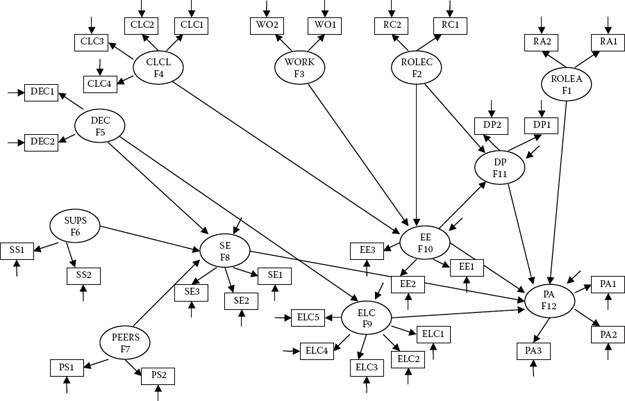
Figure 9.1. Hypothesized full SEM model of causal structure.
Mplus Input File Specification and Output File Results
Establishing the Baseline Model for the Calibration Group
Input File 1
Specification of the hypothesized model is shown in Figure 9.2. Given the known nonnormality of the data for elementary teachers, as was the case for high school teachers (see Chapter 6), the robust maximum likelihood (MLM) estimator is noted under the ANALYSIS command. Both the standardized estimates and modification indices (MIs) are requested in the OUTPUT command.
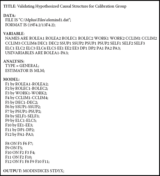
Figure 9.2. Mplus input file for test of hypothesized model of causal structure.
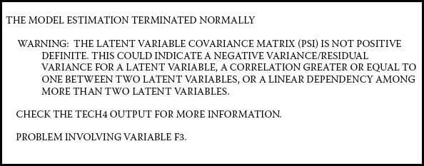
Figure 9.3. Mplus output file warning message related to test of hypothesized model.
Output File 1
Although the output file noted that estimation of the model terminated normally, this notification additionally included a warning that “the latent variable covariance matrix (psi) is not positive definite.” This matrix represents covariances among the independent factors (F1-F7) in the model. This warning message is shown in Figure 9.3, and the related estimates in Table 9.1.
As noted in the output warning message, the likely source of the problem involves Factor 3, which, as shown in Figure 9.1, represents Work (Overload), and the likely cause is either that (a) its estimated residual is negative, or (b) its correlation with another factor exceeds a value of 1.00; both problems represent what are generally known as Heywood cases1 If essence of the difficulty involves a correlation greater than 1.00, its detection is most easily found via a review of the standardized estimates. Given that the output file indicated no negative residual or factor variances, only standardized estimates for the factor correlations are reported in Table 9.1. As you can readily see, the correlation between Factors 3 and 2 exceeds a value of 1.00. This finding indicates a definite overlapping of variance between the factors of Role Conflict and Work Overload such that divergent (i.e., discriminant) validity between these two constructs is indistinctive. As such, the validity of results based on their interpretation as separate constructs is clearly dubious. Given that measurement of these two constructs derived from subscales of the same assessment scale (the Teacher Stress Scale [TSS]; Pettegrew & Wolf, 1982), this finding is not particularly uncommon but, nonetheless, needs to be addressed.
Because, in essence, the two factors of Role Conflict and Work Overload, for all intents and purposes, are representing the same construct, one approach to resolution of the difficulty is to combine these two factors into one. As such, instead of the original causal structure involving 12 factors, we would now have one representing 11 factors. This revised model is shown in Figure 9.4. Accordingly, assignment of factor numbers has been changed such that Factor 2 now represents the combined factors of ROLEC/ WORK, as measured by their original observed variables (RC1-WO2).
Table 9.1 Mplus Output: Standardized Factor Covariance Estimates

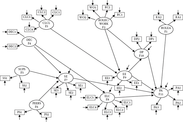
Figure 9.4. Modified hypothesized model showing constructs of role conflict and work overload combined as a single factor.

Figure 9.5. Mplus input file for test of modified model.
Input File 2
The related input file for Figure 9.4 is shown in Figure 9.5. In particular, note that the revised Factor 2 (ROLEC/WORK) is now measured by the four observed variables ROLEC1-WORK2 (RC1-WO2), and specifications regarding all remaining factors have been renumbered accordingly.
Output Files 2-4
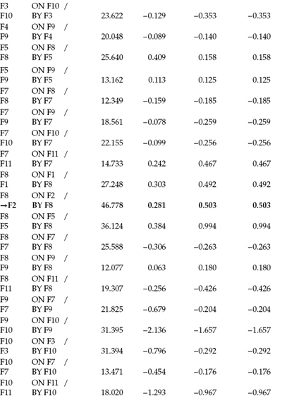
Goodness-of-fit statistics for this modified model were as follows: χ2(436) = 955.864, CFI= 0.943, RMSEA = 0.045, and SRMR = 0.060. As indicated by the CFI, RMSEA, and SRMR values, the model fit the calibration data relatively well. Nonetheless, a review of the MIs suggested that the inclusion of two additional parameters to the model, both of which were substantively reasonable, would lead to a better fitting model. The two MIs of interest here related to (a) the structural path of F8 on F2 (External Locus of Control on Role Conflict/Work Overload) and (b) a covariance between residuals associated with the observed variables EE1 and EE2, both of which are highlighted and flagged in the listing of all MI values in Table 9.2.
Consistent with my previous caveats concerning model modification based on MIs, each parameter was separately incorporated into the model and the model subsequently tested; results for each led to a (corrected) statistically significant difference from its preceding model (AMLM χ2[1] = 35.396 and AMLM χ2(1] = 29.738 , respectively). Goodness-of-fit statistics for the second of these two modified models resulted in the following: χ2(434) = 866.557, CFI= 0.953, RMSEA = 0.041, and SRMR = 0.048.
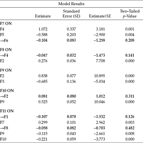
Over and above the now well-fitting model for the calibration group of elementary teachers, a review of the parameter estimates revealed five to be statistically nonsignificant. All represented structural paths in the model as follows: F7 on F6 (Self-Esteem regressed on Peer Support), F8 on F4 (External Locus of Control regressed on Decision Making), F10 on F2 (Depersonalization regressed on Role Conflict/Work Overload), F11 on F1 (Personal Accomplishment regressed on Role Ambiguity), and F11 on F8 (Personal Accomplishment regressed on External Locus of Control). Parameter estimates for all structural paths are reported in Table 9.3, with those that are nonsignificant highlighted and flagged.
In the interest of scientific parsimony, these nonsignificant paths were subsequently deleted, and the resulting model considered the established baseline model for the calibration group. As such, it serves as the model to be tested for its invariance across calibration and validation groups. However, given deletion of the paths leading from F11 to F1 and from F6 to F7, together with the fact that there are no specified relations between either F1 or F6 and any of the remaining factors, F1 and F6, most appropriately, should be deleted from the model, and the numbering of the remaining nine factors reassigned. A schematic representation of this reoriented model is shown in Figure 9.6. The dashed single-headed arrow linking the new F1 (RoleC/Work) and F6 (ELC) as well as the dashed curved arrow between EE1 and EE2 represent the newly added parameters in the model.2
Given a total restructuring of the baseline model to be used in testing for invariance across calibration and validation groups, it is important that we first review the related input file, which is presented in Figure 9.7. In addition to the change in factor number assignment, there are two essential modifications that must be made to the matching input file. First, with the removal of the constructs Role Ambiguity (ROLEA) and Peer Support (PSUP) from the model, their indicator variables (ROLEA1-ROLEA2 andPSUP1-PSUP2, respectively) will no longer be used in subsequent analyses; thus, they need to be deleted from the USEVARIABLES subcommand. Second, these four variables, likewise, will not be included in the MODEL command.
Table 9.2 Mplus Output: Selected Modification Indices


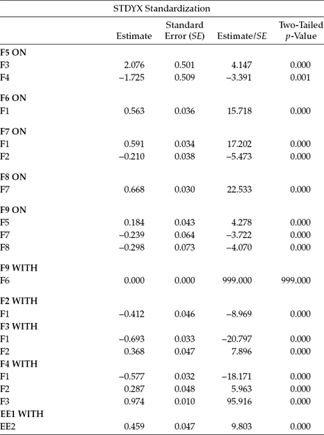
Goodness-of fit statistics for this revised baseline model were χ2(333) = 726.511, CFI = 0.950, RMSEA = 0.044, and SRMR = 0.051. However, a review of the estimated parameters revealed an estimated residual covariance between F6 and F9,3 which, of course, was not specified. In seeking the reason for this rather strange occurrence, I was advised that Mplus estimates the residual covariance between final dependent variables by default (Mplus Product Support, December 10, 2010). Of course, this unwanted parameter can be fixed to zero, and, thus, a second estimation of the baseline model was conducted with F6 with F9 constrained to 0.0. Results pertinent to this latter model were as follows: χ2(334) = 728.213, CFI = 0.950, RMSEA = 0.044, and SRMR = 0.051. Although all parameters were statistically significant, only results for the standardized structural regression paths and factor correlations are presented in Table 9.4.
Table 9.3 Mplus Output: Statistically Nonsignificant Parameters
Testing Multigroup Invariance
Having established a well-fitting and parsimonious baseline model for the calibration group, we are now ready to move on in testing for the equivalence of this causal structure across the validation group of elementary teachers. Consistent with the tests for invariance addressed in Chapters 7 and 8, our first step is to test the multigroup configural model in which no parameter constraints are specified.
Input File 1
In reviewing the input file for this configural model in Figure 9.8, you will note that, with one particular exception, the overall MODEL command reflects specification pertinent to the final baseline model for the calibration group as noted in Figure 9.7. The one exception refers to the specification of [F1-F11@0], which indicates that the factor means are constrained to a value of zero.
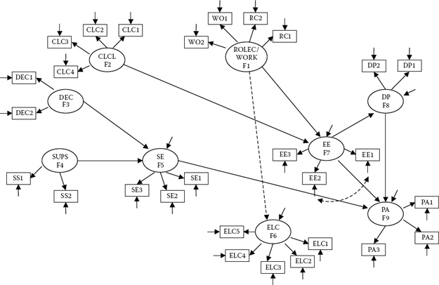
Figure 9.6. Restructured baseline model to be used in testing for invariance across calibration and validation groups.
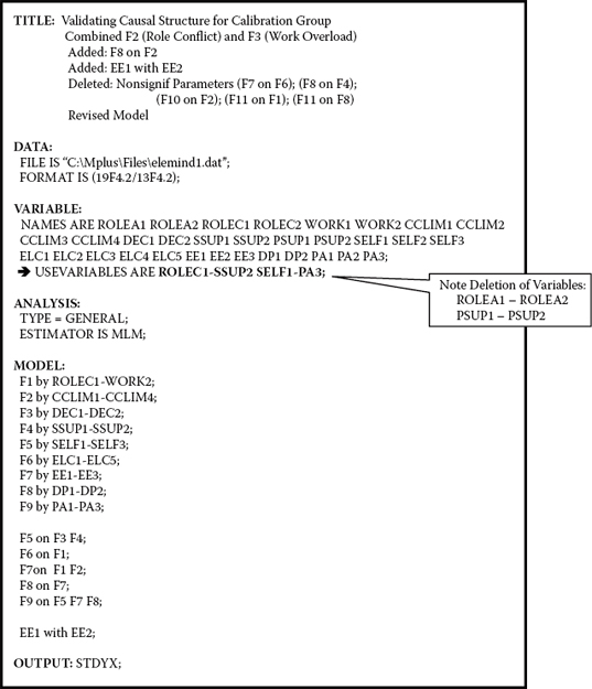
Figure 9.7. Mplus input file for restructured baseline model.
Again, consistent with multigroup model specifications in Chapters 7 and 8, the input file for the configural model also includes two model-specific commands; in the present case, one for the calibration group and one for the validation group. Recall that these model-specific command sections serve two purposes: (a) to neutralize Mplus-invoked default parameter estimation and/or equivalence across groups, and (b) to specify parameter estimation pertinent to only certain groups (i.e., not common to all groups). Because model specification for the calibration group is consistent with that shown under the overall MODEL command (i.e., there are no parameter specifications that are relevant only to the calibration group), this section remains void of specification information.
Table 9.4 Mplus Output: Standardized Parameter Estimates for Structural Regression Paths, Factor Correlations, and Residual Covariance
In contrast, the model-specific section of the input file pertinent to the validation group specifies all factor loadings and observed variable intercepts that would automatically be constrained equal by default. As mentioned above, their specification here negates their defaulted equivalence across groups. Finally, although noted in Chapters 7 and 8, I once again draw your attention to the importance of not including the reference variable loading (i.e., the factor loading constrained to 1.0 for purposes of model identification and scaling) in the model-specific section, because otherwise this parameter will be excluded from the model, thereby resulting in an error message alerting you that the model is underidentified.
Output File 1
Of import for the configural model is the extent to which it fits the data for both the calibration and validation groups simultaneously; these goodness-of-fit results are reported in Table 9.5. As you will observe from the separately reported χ2 values in this multigroup analysis, although model fit for the calibration group (χ2 = 729.143) was slightly better than it was for the validation group (χ2 = 768.829), overall model fit to their combined data yielded goodness-of-fit statistics that were negligibly different from those reported earlier for this same (baseline) model derived from the single-group analysis for the calibration group. More specifically, whereas the CFI, RMSEA, and SRMR values were 0.950, 0.044, and 0.051 respectively, when this model was tested separately for the calibration group, they remained minimally different (by only the third decimal place) when tested for both groups simultaneously.
Provided with evidence of a well-fitting model for the combined calibration and validation groups, we can now proceed with testing for the equivalence of the factor loadings, observed variable intercepts, and structural regression paths across the two groups. The input file addressing these equality constraints is presented in Figure 9.9.
Input File 2
There are several important aspects of this input file to be noted. First, given that precisely the same model is specified across groups, there are no model-specific components included in this file. Second, given that the observed variable intercepts are constrained equal by default, these parameters are not specified. Third, there are nine structural paths in the model under test, each of which will be tested for its equivalence across groups and, as such, has been assigned a specific number within parentheses. Fourth, the error covariance between EE1 and EE2 is not included in the tests for group invariance. Fifth, note that the factor means remain fixed to a value of zero and, thus, are not estimated; likewise for the default covariance between F6 and F9. Finally, I have included the specification of TECH1 in the OUTPUT command as this option is invaluable in helping you to determine if, in fact, the model has been specified as per your intent. It is particularly helpful in situations such as we have here in testing for the invariance of a full SEM model.

Figure 9.8. Mplus input file for test of configural model.
Table 9.5 Mplus Output: Selected Goodness-of-Fit Statistics for Configural Model
| Tests of Model Fit | |
| Chi-Square Test of Model Fit | |
| Value | 1497.972* |
| Degrees of freedom | 668 |
| p–value | 0.0000 |
| Scaling Correction Factor for MLM | 1.083 |
| Chi-Square Contributions From Each Group | |
| CALIBN | 729.143 |
| VALIDN | 768.829 |
| CFI/TLI | |
| CFI | 0.948 |
| TLI | 0.941 |
| Root Mean Square Error of Approximation (RMSEA) | |
| Estimate | 0.045 |
| Standardized Root Mean Square Residual (SRMR) | |
| Value | 0.056 |
Output File 2
Prior to reviewing the output results, it is perhaps instructive to first examine the difference in degrees of freedom (df) between this model in which the factor loadings, intercepts, and structural regression paths were constrained equal (df = 724) and the configural model in which these parameters were freely estimated (df = 668). Indeed, this difference of 56 is accounted for by the equating of 19 factor loadings, 28 intercepts, and 9 structural regression paths.
That these parameters were constrained equal can also be confirmed by a review of the TECH1 output. For example, the numbering of parameters in the Nu matrix (representing the observed variable intercepts) ranged from 1 through 28 inclusively, in the Lambda matrix (representing the factor loadings) from 29 through 47 inclusively, and in the Beta matrix (representing the structural regression paths) from 77 through 85 inclusively. Given that these parameters are estimated for the first group (the calibration group in the present case), albeit constrained equal for the second group, these numbers will remain the same under the TECH1 results for the validation group. That the numbers differ across the same matrices represents a clear indication that the model specification is incorrect.

Figure 9.9. Mplus input file for test of invariant factor loadings, intercepts, and structural regression paths.
Table 9.6 Mplus Output: Selected Goodness-of-Fit Statistics for Equality Constraints Model
| Tests of Model Fit | |
| Chi-Square Test of Model Fit | |
| Value | 1554.974* |
| Degrees of freedom | 724 |
| p–value | 0.0000 |
| Scaling Correction Factor for MLM | 1.082 |
| Chi-Square Contributions From Each Group | |
| CALIBN | 758.470 |
| VALIDN | 796.504 |
| CFI/TLI | |
| CFI | 0.948 |
| TLI | 0.946 |
| Root Mean Square Error of Approximation (RMSEA) | |
| Estimate | 0.044 |
| Standardized Root Mean Square Residual (SRMR) | |
| Value | 0.058 |
A review of the results related to this equality constraints model revealed both an exceptionally good fit to the data and no suggestion of potential parameter misspecification as might be indicated by the MIs. Model goodness-of-fit statistics are reported in Table 9.6.
That the CFI value remained unchanged from the one reported for the configural model speaks well for cross-group equality of the factor loadings, intercepts, and structural regression paths specified in Model 9.6. Furthermore, given that both the RMSEA and SRMR values also remain virtually unchanged (i.e., only values at the third decimal place changed), we can conclude that these parameters are operating equivalently across calibration and validation groups. Verification of these conclusions, of course, can be evidenced from computation of the corrected MLM chi-square difference test, which is found to be statistically nonsignificant (δχ2[56] = 56.172). Indeed, based on Meredith's (1993) categorization of weak, strong, and strict invariance, these results would indicate clear evidence of strong measurement and structural invariance.
Notes
| 1. | Heywood cases represent out-of-range estimated values such as negative error (i.e., residual) variances and correlations greater than 1.00. |
| 2. | Deletion of these parameters could also be accomplished in two alternative ways: (a) by fixing each of the nonsignificant paths to zero, or (b) by simply not estimating the nonsignificant paths. Both approaches, however, result in a less parsimonious model than the one shown in Figure 9.6 and tested here. In addition, be aware that estimation of the model via the (b) approach leads to a difference of four degrees of freedom, rather than five, due to the Mplus default noted here with the reoriented model. |
| 3. | We know this parameter represents a residual covariance and not a factor variance as only the covariances of independent continuous factors in the model are estimated by default. |