
Chapter 10 – OLAP Functions
“Don’t count the days, make the days count.”
- Mohammed Ali
The Row_Number Command
SELECT Product_ID ,Sale_Date , Daily_Sales,
ROW_NUMBER() OVER
(ORDER BY Product_ID, Sale_Date) AS Seq_Number
FROM Sales_Table WHERE Product_ID IN (1000, 2000) ;

The ROW_NUMBER Keyword(s) caused Seq_Number to increase sequentially. Notice that this does NOT have a Rows Unbounded Preceding, and it still works!
Quiz – How did the Row_Number Reset?
SELECT Product_ID ,Sale_Date , Daily_Sales,
ROW_NUMBER() OVER (PARTITION BY Product_ID
ORDER BY Product_ID, Sale_Date ) AS StartOver
FROM Sales_Table WHERE Product_ID IN (1000, 2000) ;

What Keyword(s) caused StartOver to reset?
Quiz – How did the Row_Number Reset?
SELECT Product_ID ,Sale_Date , Daily_Sales,
ROW_NUMBER() OVER (PARTITION BY Product_ID
ORDER BY Product_ID, Sale_Date ) AS StartOver
FROM Sales_Table WHERE Product_ID IN (1000, 2000) ;

What Keyword(s) caused StartOver to reset? It is the PARTITION BY statement.
Using a Derived Table and Row_Number
WITH Results AS
( SELECT
ROW_NUMBER()
OVER(ORDER BY Product_ID, Sale_Date) AS RowNumber,
Product_ID, Sale_Date
FROM Sales_Table
)
SELECT *
FROM Results
WHERE RowNumber BETWEEN 8 AND 14

In the example above we are using a derived table called Results and then using a WHERE clause to only take certain RowNumbers.
Finding the First Occurrence using a WITH Derived Table

Using the Row_Number ordered analytic and by partitioning of Product_ID and the sorting by Sale_Date ASC we are bringing back only the first occurrence of a row based on the earliest Sale_Date. This can be done because we are placing our query in a derived table and then selecting from that derived table using a WHERE clause.
Finding the Last Occurrence using a WITH Derived Table

Using the Row_Number ordered analytic and by partitioning of Product_ID and the sorting by Sale_Date DESC we are bringing back only the first occurrence of a row based on the latest Sale_Date. This can be done because we are placing our query in a derived table and then selecting from that derived table using a WHERE clause.
Ordered Analytics OVER
SELECT
Product_ID as Prod ,Sale_Date ,Daily_Sales
,SUM(Daily_Sales) OVER(PARTITION BY Sale_Date) AS Total
,AVG(Daily_Sales) OVER(PARTITION BY Sale_Date) AS Avg
,COUNT(Daily_Sales) OVER(PARTITION BY Sale_Date) AS Cnt
,MIN(Daily_Sales) OVER(PARTITION BY Sale_Date) AS Min
,MAX(Daily_Sales) OVER(PARTITION BY Sale_Date) AS Max
FROM Sales_Table

Not all rows are shown in the answer set
Above is an example of the Ordered Analytics that uses the keyword OVER.
RANK and DENSE RANK
SELECT
Product_ID,
Daily_Sales,
RANK() OVER (ORDER BY Daily_Sales ASC) as "Rank",
DENSE_RANK() OVER(Order By Daily_Sales ASC) as "DenseRank"
FROM Sales_Table
WHERE Product_ID in(1000, 2000)

Above is an example of the RANK and DENSE_RANK commands. Notice the difference in the ties and the next ranking.
RANK Defaults to Ascending Order
SELECT Product_ID ,Sale_Date , Daily_Sales,
RANK() OVER (ORDER BY Daily_Sales) AS Rank1
FROMSales_Table
WHERE Product_ID IN (1000, 2000) ;

The RANK OVER command defaults the Sort to ASC.
Getting RANK to Sort in DESC Order
SELECT Product_ID ,Sale_Date , Daily_Sales,
RANK() OVER (ORDER BY Daily_Sales DESC)
AS Rank1
FROM Sales_Table WHERE Product_ID IN (1000, 2000) ;

Utilize the DESC keyword in the ORDER BY statement to rank in descending order.
RANK OVER and PARTITION BY
SELECT Product_ID ,Sale_Date , Daily_Sales,
RANK() OVER (PARTITION BY Product_ID
ORDER BY Daily_Sales DESC) AS Rank1
FROM Sales_Table WHERE Product_ID IN (1000, 2000) ;

What does the PARTITION Statement in the RANK OVER do? It resets the rank.
PERCENT_RANK OVER
SELECT Product_ID ,Sale_Date , Daily_Sales,
PERCENT_RANK() OVER (PARTITION BY PRODUCT_ID
ORDER BY Daily_Sales DESC) AS PercentRank1
FROM Sales_Table WHERE Product_ID in (1000, 2000) ;
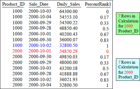
We now have added a Partition statement which resets on Product_ID so this produces 7 rows for each of our Product_IDs.
PERCENT_RANK OVER with 14 rows in Calculation
SELECT Product_ID ,Sale_Date , Daily_Sales,
PERCENT_RANK()
OVER ( ORDER BY Daily_Sales DESC) AS PercentRank1
FROM Sales_Table WHERE Product_ID IN (1000, 2000) ;
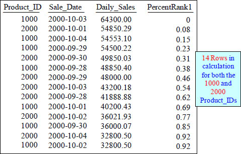
Percent_Rank is just like RANK, however, it gives you the Rank as a percent, but only a percent of all the other rows up to 100%.
PERCENT_RANK OVER with 21 rows in Calculation
SELECT Product_ID ,Sale_Date , Daily_Sales,
PERCENT_RANK() OVER ( ORDER BY Daily_Sales DESC)
AS PercentRank1
FROM Sales_Table ;

Percent_Rank is just like RANK, however, it gives you the Rank as a percent but only a percent of all the other rows up to 100%.
Quiz – What Causes the Product_ID to Reset?
SELECT Product_ID ,Sale_Date , Daily_Sales,
PERCENT_RANK() OVER (PARTITION BY PRODUCT_ID
ORDER BY Daily_Sales DESC) AS PercentRank1
FROM Sales_Table WHERE Product_ID in (1000, 2000) ;

What caused the Product_IDs to be sorted?
Answer to Quiz – What Cause the Product_ID to Reset?
SELECT Product_ID ,Sale_Date , Daily_Sales,
PERCENT_RANK() OVER (PARTITION BY PRODUCT_ID
ORDER BY Daily_Sales DESC) AS PercentRank1
FROMSales_Table WHERE Product_ID in (1000, 2000) ;

What caused the Product_IDs to be sorted? It was the PARTITION BY statement.
Finding Gaps between Dates
SELECT Product_Id, Sale_Date,
MIN(Sale_Date) OVER (PARTITION BY Product_Id
ORDER BY Sale_Date ROWS BETWEEN 1 FOLLOWING
AND UNBOUNDED FOLLOWING) AS Date_Of_Next_Row
,MIN(Sale_Date) OVER (PARTITION BY Product_Id
ORDER BY Sale_Date
ROWS BETWEEN 1 FOLLOWING
AND UNBOUNDED FOLLOWING) - Sale_Date AS Days_To_Next_Row
FROM Sales_Table WHERE Product_ID Between 1000 and 2000 ;

The above query finds gaps in dates.
CSUM – Rows Unbounded Preceding Explained
SELECT Product_ID , Sale_Date, Daily_Sales,
SUM(Daily_Sales) OVER (ORDER BY Sale_Date
ROWS UNBOUNDED PRECEDING) AS CsumAnsi
FROM Sales_Table
WHERE Product_ID BETWEEN 1000 and 2000 ;

The keywords Rows Unbounded Preceding determines that this is a cumulative sum (CSUM). There are only a few different statements and Rows Unbounded Preceding is the main one. It means start calculating at the beginning row, and continue calculating until the last row.
CSUM – Making Sense of the Data
SELECT Product_ID , Sale_Date, Daily_Sales,
SUM(Daily_Sales) OVER (ORDER BY Sale_Date
ROWS UNBOUNDED PRECEDING) AS SUMOVER
FROM Sales_Table WHERE Product_ID BETWEEN 1000 and 2000 ;

The second “SUMOVER” row is 90739.28. That is derived by the first row’s Daily_Sales (41888.88) added to the SECOND row’s Daily_Sales (48850.40).
CSUM – Making Even More Sense of the Data
SELECT Product_ID , Sale_Date, Daily_Sales,
SUM(Daily_Sales) OVER (ORDER BY Sale_Date
ROWS UNBOUNDED PRECEDING) AS SUMOVER
FROM Sales_Table WHERE Product_ID BETWEEN 1000 and 2000 ;

The third “SUMOVER” row is 138739.28. That is derived by taking the first row’s Daily_Sales (41888.88) and adding it to the SECOND row’s Daily_Sales (48850.40). Then, you add that total to the THIRD row’s Daily_Sales (48000.00).
CSUM – The Major and Minor Sort Key(s)
SELECT Product_ID , Sale_Date, Daily_Sales,
SUM(Daily_Sales) OVER (ORDER BY Product_ID, Sale_Date
ROWS UNBOUNDED PRECEDING) AS SumOVER
FROM Sales_Table ;

You can have more than one SORT KEY. In the top query, Product_ID is the MAJOR Sort and Sale_Date is the MINOR Sort. Remember, the data is sorted first and then the cumulative sum is calculated. That is why they are called Ordered Analytics.
The ANSI CSUM – Getting a Sequential Number
SELECT Product_ID , Sale_Date, Daily_Sales,
SUM(Daily_Sales) OVER (ORDER BY Product_ID, Sale_Date
ROWS UNBOUNDED PRECEDING) as SUMOVER,
SUM(1) OVER (ORDER BY Product_ID, Sale_Date
↑ ROWS UNBOUNDED PRECEDING) AS Seq_Number
FROM Sales_Table ;

With “Seq_Number”, it will continuously add 1 to the answer for each row. Because you placed the number 1 in the area which calculates the cumulative sum, it will continuously add 1 to the answer for each row.
Troubleshooting the ANSI OLAP on a GROUP BY
SELECT Product_ID , Sale_Date, Daily_Sales,
SUM(Daily_Sales) OVER (ORDER BY Sale_Date
ROWS UNBOUNDED PRECEDING) AS AnsiCsum
FROM Sales_Table
GROUP BY Product_ID ;
Error! Why?
Never GROUP BY in a SUM Over or with any ANSI Syntax OLAP command. If you want to reset, use a PARTITION BY Statement, but never a GROUP BY.
Reset with a PARTITION BY Statement
SELECT Product_ID , Sale_Date, Daily_Sales,
SUM(Daily_Sales) OVER (PARTITION BY Product_ID
ORDER BY Product_ID, Sale_Date
ROWS UNBOUNDED PRECEDING) AS SumANSI
FROM Sales_Table ;

The PARTITION Statement is how you reset in ANSI. This will cause the SUMANSI to start over (reset) on its calculating for each NEW Product_ID.
PARTITION BY only Resets a Single OLAP not ALL of them
SELECT Product_ID , Sale_Date, Daily_Sales,
SUM(Daily_Sales) OVER (PARTITION BY Product_ID
ORDER BY Product_ID, Sale_Date
ROWS UNBOUNDED PRECEDING) AS Subtotal,
SUM(Daily_Sales) OVER (ORDER BY Product_ID, Sale_Date
ROWS UNBOUNDED PRECEDING) AS GrandTotal
FROM Sales_Table ;
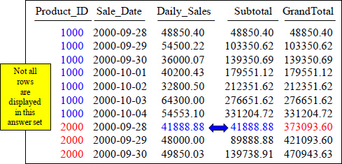
Above are two OLAP statements. Only one has PARTITION BY, so only it resets. The other continuously does a CSUM.
CURRENT ROW AND UNBOUNDED FOLLOWING
SELECT Product_ID, Sale_Date ,Daily_Sales
,SUM(Daily_Sales) OVER (ORDER BY Product_ID, Sale_Date
ROWS BETWEEN CURRENT ROW AND UNBOUNDED FOLLOWING)
AS CumulativeTotal
FROM Sales_Table
ORDER BY CumulativeTotal

Above we used the ROWS BETWEEN CURRENT ROW AND UNBOUNDED FOLLOWING to produce a CSUM, but notice that the Product_ID and the Sale_Date are reversed. We see the Product_ID of 3000 first and the latest date first.
Different Windowing Options
SELECT Product_ID, Sale_Date, Daily_Sales
,SUM(Daily_Sales)
OVER( PARTITION BY Product_ID ORDER BY Product_ID, Sale_Date
ROWS BETWEEN 1 PRECEDING AND CURRENT ROW ) as Row_Preceding
,SUM(Daily_Sales)
OVER( PARTITION BY Product_ID ORDER BY Product_Id, Sale_Date
ROWS BETWEEN CURRENT ROW AND 1 FOLLOWING) as Row_Following
FROM Sales_Table

The example above uses ROWS BETWEEN 1 PRECEDING AND CURRENT ROW and then uses a different example with ROWS BETWEEN CURRENT ROW AND 1 FOLLOWING. Notice how the report came out?
Moving Sum has a Moving Window

The SUM () Over allows you to get the moving SUM of a certain column. The moving window in ANSI form always includes the current row. A Rows 2 Preceding statement means the current row and two preceding, which is a moving window of 3.
How ANSI Moving SUM Handles the Sort

The SUM OVER places the sort after the ORDER BY.
Quiz – How is that Total Calculated?
SELECT Product_ID , Sale_Date, Daily_Sales,
SUM(Daily_Sales) OVER (ORDER BY Product_ID, Sale_Date
ROWS 2 Preceding) AS Sum3_ANSI
FROM Sales_Table ;

With a Moving Window of 3, how is the 139350.69 amount derived in the Sum3_ANSI column in the third row?
Answer to Quiz – How is that Total Calculated?
SELECT Product_ID , Sale_Date, Daily_Sales,
SUM(Daily_Sales) OVER (ORDER BY Product_ID, Sale_Date
ROWS 2 Preceding) AS Sum3_ANSI
FROM Sales_Table ;

With a Moving Window of 3, how is the 139350.69 amount derived in the Sum3_ANSI column in the third row? It is the sum of 48850.40, 54500.22 and 36000.07. The current row of Daily_Sales plus the previous two rows of Daily_Sales.
Moving SUM every 3-rows Vs a Continuous Average
SELECT Product_ID , Sale_Date, Daily_Sales,
SUM(Daily_Sales) OVER (ORDER BY Product_ID, Sale_Date
ROWS 2 Preceding) AS SUM3,
SUM(Daily_Sales) OVER (ORDER BY Product_ID, Sale_Date
ROWS UNBOUNDED Preceding) AS Continuous
FROM Sales_Table;

Not all rows are displayed in this answer set
The ROWS 2 Preceding gives the MSUM for every 3 rows. The ROWS UNBOUNDED Preceding gives the continuous MSUM.
PARTITION BY Resets an ANSI OLAP

Use a PARTITION BY Statement to Reset the ANSI OLAP. Notice it only resets the OLAP command containing the Partition By statement, but not the other OLAPs.
The Moving Window is Current Row and Preceding

The AVG () Over allows you to get the moving average of a certain column. The Rows 2 Preceding is a moving window of 3 in ANSI.
How Moving Average Handles the Sort

Much like the SUM OVER Command, the Average OVER places the sort keys via the ORDER BY keywords.
Moving Average
SELECT Product_ID , Sale_Date, Daily_Sales,
AVG(Daily_Sales) OVER (ORDER BY Product_ID, Sale_Date
ROWS 2 Preceding) AS AVG_3
FROM Sales_Table ;

Understand that in ANSI a ROWS 2 PRECEDING is considered a Moving Window of 3. That is because in ANSI it is considered the Current Row and 2 preceding. The next page will use the CAST command to provide a precision of 0 decimal places.
Moving Average

Understand that in ANSI a ROWS 2 PRECEDING is considered a Moving Window of 3. That is because in ANSI it is considered the Current Row and 2 preceding.
Quiz – How is that Total Calculated?
SELECT Product_ID , Sale_Date, Daily_Sales,
AVG(Daily_Sales) OVER (ORDER BY Product_ID, Sale_Date
ROWS 2 Preceding) AS AVG_3_ANSI
FROM Sales_Table ;

With a Moving Window of 3, how is the 46450.23 amount derived in the AVG_3_ANSI column in the third row?
Answer to Quiz – How is that Total Calculated?
SELECT Product_ID , Sale_Date, Daily_Sales,
AVG(Daily_Sales) OVER (ORDER BY Product_ID, Sale_Date
ROWS 2 Preceding) AS AVG_3_ANSI
FROM Sales_Table ;

AVG of 48850.40, 54500.22, and 36000.07
With a Moving Window of 3, the 46450.23 amount derived in the third row is the average of 48850.40, 54500.22 and 36000.07.
Quiz – How is that 4th Row Calculated?
SELECT Product_ID , Sale_Date, Daily_Sales,
AVG(Daily_Sales) OVER (ORDER BY Product_ID, Sale_Date
ROWS 2 Preceding) AS AVG_3_ANSI
FROM Sales_Table ;

With a Moving Window of 3, how is the 43566.91 amount derived in the AVG_3_ANSI column in the fourth row?
Answer to Quiz – How is that 4th Row Calculated?
SELECT Product_ID , Sale_Date, Daily_Sales,
AVG(Daily_Sales) OVER (ORDER BY Product_ID, Sale_Date
ROWS 2 Preceding) AS AVG_3_ANSI
FROM Sales_Table ;

AVG of 54500.22, 36000.07 and 40200.43
With a Moving Window of 3, how is the 43566.91 amount derived in the AVG_3_ANSI column in the fourth row? The current row plus Rows 2 Preceding.
Moving Average every 3-rows vs a Continuous Average
SELECT Product_ID , Sale_Date, Daily_Sales,
AVG(Daily_Sales) OVER (ORDER BY Product_ID, Sale_Date
ROWS 2 Preceding) AS AVG3,
AVG(Daily_Sales) OVER (ORDER BY Product_ID, Sale_Date
ROWS UNBOUNDED Preceding) AS Continuous
FROM Sales_Table;

The ROWS 2 Preceding gives the MAVG for every 3 rows. The ROWS UNBOUNDED Preceding gives the continuous MAVG.
PARTITION BY Resets an ANSI OLAP

Use a PARTITION BY Statement to Reset the ANSI OLAP. The Partition By statement only resets the column using the statement. Notice that only Continuous resets.
Moving Difference using ANSI Syntax
SELECT Product_ID, Sale_Date, Daily_Sales,
Daily_Sales - SUM(Daily_Sales)
OVER ( ORDER BY Product_ID ASC, Sale_Date ASC
ROWS BETWEEN 4 PRECEDING AND 4 PRECEDING)
AS "MDiff_ANSI"
FROM Sales_Table ;

This is how you do a MDiff using the ANSI Syntax with a moving window of 4.
Moving Difference using ANSI Syntax with Partition By
SELECT Product_ID, Sale_Date, Daily_Sales,
Daily_Sales - SUM(Daily_Sales) OVER (PARTITION BY Product_ID
ORDER BY Product_ID ASC, Sale_Date ASC
ROWS BETWEEN 4 PRECEDING AND 4 PRECEDING) AS "MDiff_ANSI"
FROM Sales_Table;

Wow! This is how you do a MDiff using the ANSI Syntax with a moving window of 4 and with a PARTITION BY statement.
COUNT OVER for a Sequential Number
SELECT Product_ID ,Sale_Date , Daily_Sales,
COUNT(*) OVER (ORDER BY Product_ID, Sale_Date
ROWS UNBOUNDED PRECEDING) AS Seq_Number
FROMSales_Table WHERE Product_ID IN (1000, 2000) ;

This is the COUNT OVER. It will provide a sequential number starting at 1. The Keyword(s) ROWS UNBOUNDED PRECEDING causes Seq_Number to start at the beginning and increase sequentially to the end.
COUNT OVER without Rows Unbounded Preceding
SELECT Product_ID ,Sale_Date , Daily_Sales,
COUNT(*) OVER (ORDER BY Product_ID, Sale_Date) AS No_Seq
FROM Sales_Table WHERE Product_ID IN (1000, 2000) ;

When you don’t have a ROWS UNBOUNDED PRECEDING this still works just fine.
Quiz – What caused the COUNT OVER to Reset?
SELECT Product_ID ,Sale_Date , Daily_Sales,
COUNT(*) OVER (PARTITION BY Product_ID
ORDER BY Product_ID, Sale_Date
ROWS UNBOUNDED PRECEDING) AS StartOver
FROM Sales_Table WHERE Product_ID IN (1000, 2000) ;

What Keyword(s) caused StartOver to reset?
Answer to Quiz – What caused the COUNT OVER to Reset?
SELECT Product_ID ,Sale_Date , Daily_Sales,
COUNT(*) OVER (PARTITION BY Product_ID
ORDER BY Product_ID, Sale_Date
ROWS UNBOUNDED PRECEDING) AS StartOver
FROM Sales_Table WHERE Product_ID IN (1000, 2000) ;

What Keyword(s) caused StartOver to reset? It is the PARTITION BY statement.
The MAX OVER Command
SELECT Product_ID ,Sale_Date , Daily_Sales,
MAX(Daily_Sales) OVER (ORDER BY Product_ID, Sale_Date
ROWS UNBOUNDED PRECEDING) AS MaxOver
FROM Sales_Table WHERE Product_ID IN (1000, 2000) ;

After the sort, the Max Over shows the Max Value up to that point.
MAX OVER with PARTITION BY Reset
SELECT Product_ID ,Sale_Date , Daily_Sales,
MAX(Daily_Sales) OVER (PARTITION BY Product_ID
ORDER BY Product_ID, Sale_Date
ROWS UNBOUNDED PRECEDING) AS MaxOver
FROM Sales_Table WHERE Product_ID IN (1000, 2000) ;

The largest value is 64300.00 in the column MaxOver. Once it was evaluated, it did not continue until the end because of the PARTITION BY reset.
MAX OVER without Rows Unbounded Preceding
SELECT Product_ID ,Sale_Date , Daily_Sales,
MAX(Daily_Sales) OVER (ORDER BY Product_ID, Sale_Date )
AS MaxOver
FROM Sales_Table WHERE Product_ID IN (1000, 2000) ;

You don't need the Rows Unbounded Preceding with the MAX OVER.
The MIN OVER Command
SELECT Product_ID, Sale_Date ,Daily_Sales
,MIN(Daily_Sales) OVER (ORDER BY Product_ID, Sale_Date
ROWS UNBOUNDED PRECEDING) AS MinOver
FROM Sales_Table WHERE Product_ID IN (1000, 2000) ;

After the sort, the MIN () Over shows the Max Value up to that point.
MIN OVER without Rows Unbounded Preceding
SELECT Product_ID ,Sale_Date , Daily_Sales,
MIN(Daily_Sales) OVER (ORDER BY Product_ID, Sale_Date )
AS MinOver
FROM Sales_Table WHERE Product_ID IN (1000, 2000) ;

You don't need the Rows Unbounded Preceding with the MIN OVER.
Finding a Value of a Column in the Next Row with MIN
SELECT Product_ID, Sale_Date, Daily_Sales,
MIN(Daily_Sales) OVER (PARTITION BY Product_ID
ORDER BY Product_ID, Sale_Date
ROWS BETWEEN 1 Following and 1 Following) AS NextSale
FROM Sales_Table WHERE Product_ID IN (1000, 2000) ;

The above example finds the value of a column in the next row for Daily_Sales. Notice it is partitioned so there is a Null value at the end of each Product_ID.
The CSUM for Each Product_Id and the Next Start Date
SELECT ROW_NUMBER() OVER (PARTITION BY Product_ID
ORDER BY Sale_Date) As Rnbr
,Product_Id as PROD ,Sale_Date
,MIN(Sale_Date)OVER (PARTITION BY Product_ID
ORDER BY Sale_Date ROWS BETWEEN 1 FOLLOWING
AND 1 FOLLOWING) As Next_Start_Dt
,Daily_Sales
,SUM(Daily_Sales) OVER (PARTITION BY Product_ID
ORDER BY Sale_Date ROWS UNBOUNDED PRECEDING)
As To_Date_RevenueFROM Sales_Table

The above example shows the cumulative SUM for the Daily_Sales and the next date on the same line.
Quiz – Fill in the Blank
SELECT Product_ID ,Sale_Date , Daily_Sales,
MIN(Daily_Sales)OVER (PARTITION BY Product_ID
ORDER BY Product_ID, Sale_Date
ROWS UNBOUNDED PRECEDING) AS MinOver
FROM Sales_Table WHERE Product_ID IN (1000, 2000) ;

The last two answers (MinOver) are blank, so you can fill in the blank.
Answer – Fill in the Blank
SELECT Product_ID ,Sale_Date , Daily_Sales,
MIN(Daily_Sales)OVER (PARTITION BY Product_ID
ORDER BY Product_ID, Sale_Date
ROWS UNBOUNDED PRECEDING) AS MinOver
FROM Sales_Table WHERE Product_ID IN (1000, 2000) ;

The last two answers (MinOver) are filled in.
How Ntile Works
SELECTProduct_ID, Sale_Date, Daily_Sales
,NTILE (4) OVER (ORDER BY Daily_Sales , Sale_Date ) AS "Quartiles"
FROMSales_Table WHERE Product_ID = 1000;

Assigning a different value to the <partitions> indicator of the Ntile function changes the number of partitions established. Each Ntile partition is assigned a number starting at 1 increasing to a value that is one less than the partition number specified. So, with an Ntile of 4 the partitions are 1 through 4. Then, all the rows are distributed as evenly as possible into each partition from highest to lowest values. Normally, extra rows with the lowest value begin back in the lowest numbered partitions.
Ntile
SELECT Last_Name,Grade_Pt,
NTILE(5) OVER (ORDER BY Grade_Pt) as "Tile"
FROM Student_Table
ORDER BY "Tile" DESC;

The Ntile function organizes rows into n number of groups. These groups are referred to as tiles. The tile number is returned. For example, the example above has 10 rows, so NTILE (5) splits the 10 rows into five equally sized tiles. There are 2 rows in each tile in the order of the OVER clause's ORDER BY.
Ntile Continued
SELECT Dept_No, EmployeeCount,
NTILE(2) OVER (ORDER BY EmployeeCount) as "Tile"
FROM (SELECT Dept_No, COUNT(*) as EmployeeCount
FROM Employee_Table
GROUP BY Dept_No
) AS Q
ORDER BY "Tile" DESC;

The Ntile function organizes rows into n number of groups. These groups are referred to as tiles. The tile number is returned. For example, the example above has 6 rows, so NTILE (2) splits the 10 rows into 2 equally sized tiles. There are 3 rows in each tile in the order of the OVER clause's ORDER BY.
Ntile Percentile
SELECT Claim_ID, Claim_Date, ClaimCount,
NTILE(100) OVER (ORDER BY ClaimCount) as Percentile
FROM (SELECT Claim_ID, Claim_Date, COUNT(*) as ClaimCount
FROM Claims
GROUP BY Claim_ID, Claim_Date
) AS Q
ORDER BY Percentile DESC

The Ntile function organizes rows into n number of groups. These groups are referred to as tiles. The tile number is returned. Above is a way to get the percentile.
Another Ntile Example
This example determines the percentile for every row in the Sales
table based on the daily sales amount and sorts it into sequence
by the value being categorized, which here is daily sales.
SELECT Product_ID, Sale_Date, Daily_Sales
,NTILE(100) OVER (ORDER BY Daily_Sales) AS "Quantile"
FROMSales_Table
WHERE Product_ID < 2000 ;

Above is another Ntile example.
Using Tertiles (Partitions of Four)
SELECT Product_ID, Sale_Date, Daily_Sales
,NTILE (4) OVER (Order by Daily_Sales , Sale_Date ) AS "Quartiles"
FROM Sales_Table WHERE Product_ID in (1000, 2000) ;

Instead of 100, the example above uses a quartile (QUANTILE based on 4 partitions).
NTILE
SELECT Product_ID ,Sale_Date , Daily_Sales,
NTILE(4) OVER (ORDER BY Daily_Sales) AS Bucket
FROM Sales_Table WHERE Product_ID IN (1000, 2000) ;

The NTILE function divides the rows into buckets as evenly as possible. In this example, because PARTITION BY is omitted, the entire input will be sorted using the ORDER BY clause, and then divided into the number of buckets specified.
NTILE Using a Value of 10
SELECT Product_ID ,Sale_Date , Daily_Sales,
NTILE(10) OVER (ORDER BY Daily_Sales) AS Bucket
FROM Sales_Table WHERE Product_ID IN (1000, 2000) ;

The NTILE function divides the rows into buckets as evenly as possible. In this example, because PARTITION BY is omitted, the entire input will be sorted using the ORDER BY clause, and then divided into the number of buckets specified. This example uses a value of 10 in the NTILE.
NTILE with a Partition
SELECT Product_ID ,Sale_Date , Daily_Sales,
NTILE(3) OVER (PARTITION BY Product_ID
ORDER BY Daily_Sales) AS Bucket
FROM Sales_Table WHERE Product_ID IN (1000, 2000) ;

The NTILE function divides the rows into buckets as evenly as possible. In this example, because PARTITION BY is listed, the data will first be sorted by Product_ID and then sorted using the ORDER BY clause (within Product_ID), and then divided into the number of buckets specified. This example uses a value of 3 in the NTILE. Notice that the PARTITION BY statement causes the answer set to reset on Product_ID breaks.
Using FIRST_VALUE
SELECT Last_name, first_name, dept_no
,FIRST_VALUE(first_name)
OVER (ORDER BY dept_no, last_name desc
rows unbounded preceding) AS "First All"
,FIRST_VALUE(first_name)
OVER (PARTITION BY dept_no
ORDER BY dept_no, last_name desc
rows unbounded preceding)
AS "First Partition"
FROM Employee_Table;

The above example uses FIRST_VALUE to show you the very first first_name returned. It also uses the keyword Partition to show you the very first first_name returned in each department.
FIRST_VALUE
SELECT Product_ID ,Sale_Date , Daily_Sales,
Daily_Sales - First_Value (Daily_Sales)
OVER (ORDER BY Sale_Date) AS Delta_First
FROM Sales_Table WHERE Product_ID IN (1000, 2000) ;

Above, after sorting the data by Sale_Date, we compute the difference between the first row's Daily_Sales and the Daily_Sales of each following row. All rows Daily_Sales are compared with the first row's Daily_Sales, thus the name First_Value.
FIRST_VALUE after Sorting by the Highest Value
SELECT Product_ID ,Sale_Date , Daily_Sales,
Daily_Sales - First_Value (Daily_Sales)
OVER (ORDER BY Daily_Sales DESC)AS Delta_First
FROM Sales_Table WHERE Product_ID IN (1000, 2000) ;

Above, after sorting the data by Daily_Sales DESC, we compute the difference between the first row's Daily_Sales and the Daily_Sales of each following row. All rows Daily_Sales are compared with the first row's Daily_Sales, thus the name First_Value. This example shows that how much less each Daily_Sales is compared to 64,300.00 (our highest sale).
FIRST_VALUE with Partitioning
SELECT Product_ID ,Sale_Date , Daily_Sales,
Daily_Sales - First_Value (Daily_Sales)
OVER (PARTITION BY Product_ID
ORDER BY Sale_Date) AS Delta_First
FROMSales_Table WHERE Product_ID IN (1000, 2000) ;

We are now comparing the Daily_Sales of the first Sale_Date for each Product_ID with the Daily_Sales of all other rows within the Product_ID partition. Each row is only compared with the first row (First_Value) in it's partition.
Using LAST_VALUE
SELECT Last_name, first_name, dept_no
,LAST_VALUE(first_name)
OVER (ORDER BY dept_no, last_name desc
rows unbounded preceding)AS "Last All"
,LAST_VALUE(first_name)
OVER (PARTITION BY dept_no
ORDER BY dept_no, last_name desc
rows unbounded preceding) AS "Last Partition"
FROMsql_class.Employee_Table;

The FIRST_VALUE and LAST_VALUE are good to use anytime you need to propagate a value from one row to all or multiple rows based on a sorted sequence. However, the output from the LAST_VALUE function appears to be incorrect and is a little misleading until you understand a few concepts. The SQL request specifies "rows unbounded preceding“, and LAST_VALUE looks at the last row. The current row is always the last row, and therefore, it appears in the output.
LAST_VALUE
SELECT Product_ID ,Sale_Date , Daily_Sales,
Daily_Sales - LAST_Value (Daily_Sales)
OVER (ORDER BY Sale_Date) AS Delta_Last
FROMSales_Table WHERE Product_ID IN (1000, 2000) ;
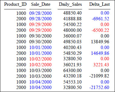
Above, after sorting the data by Sale_Date, we compute the difference between the last row's Daily_Sales and the Daily_Sales of each following row (from the same Sale_Date). Since there is only two product totals for each day, there is always a 0.00 for one of the rows.
Using LAG and LEAD
Compatibility: Vertica Extension
The LAG and LEAD functions allow you to compare different rows of a table by specifying an offset from the current row. You can use these functions to analyze change and variation.
Syntax for LAG and LEAD:
{LAG | LEAD} (<value expression>, [<offset> [, <default>]]) OVER
([PARTITION BY <column reference>[,...]]
ORDER BY <column reference> [ASC | DESC] [,...] ) ;
The above provides information and the syntax for LAG and LEAD.
Using LEAD
SELECT
Last_Name, Dept_No
,LEAD(Dept_No)
OVER (ORDER BY Dept_No, Last_Name) as "Lead All"
,LEAD(Dept_No) OVER (PARTITION BY Dept_No
ORDER BY Dept_No, Last_Name) as "Lead Partition"
FROM Employee_Table;

As you can see, the first LEAD brings back the value from the next row except for the last which has no row following it. The offset value was not specified in this example, so it defaulted to a value of 1 row.
Using LEAD With and Offset of 2
SELECT Last_Name, Dept_No
,LEAD(Dept_No,2)
OVER (ORDER BY Dept_No, Last_Name) as "Lead All"
,LEAD(Dept_No,2)
OVER (PARTITION BY Dept_No
ORDER BY Dept_No, Last_Name) as "Lead Partition"
FROM Employee_Table;

Above, each value in the first LEAD is 2 rows away, and the partitioning only shows when values are contained in each value group with 1 more than offset value.
LEAD
SELECT Product_ID ,Sale_Date , Daily_Sales,
Daily_Sales - LEAD(Daily_Sales, 1, 0)
OVER (ORDER BY Product_ID, Sale_Date) AS Lead1
FROM Sales_Table WHERE Product_ID IN (1000, 2000) ;

Above, we compute the difference between a product's Daily_Sales and that of the next Daily_Sales in the sort order (which will be the next row's Daily_Sales, or one whose Daily_Sales is the same). The expression LEAD (Daily_Sales, 1, 0) tells LEAD () to evaluate the expression Daily_Sales on the row that is positioned one row following the current row. If there is no such row (as is the case on the last row of the partition or relation), then the default value of 0 is used.
LEAD With Partitioning
SELECT Product_ID ,Sale_Date , Daily_Sales,
Daily_Sales - LEAD(Daily_Sales, 1, 0)
OVER (PARTITION BY Product_ID ORDER BY Sale_Date) AS Lead1
FROM Sales_Table WHERE Product_ID IN (1000, 2000) ;

Above, we compute the difference between a product's Daily_Sales and that of the next Daily_Sales in the sort order (which will be the next row's Daily_Sales, or one whose Daily_Sales is the same). We also partitioned the data by Product_ID.
Using LAG
SELECT Last_Name, Dept_No
,LAG(Dept_No)
OVER (ORDER BY Dept_No, Last_Name) as "Lag All"
,LAG(Dept_No)
OVER (PARTITION BY Dept_No
ORDER BY Dept_No, Last_Name) as "Lag Partition"
FROM Employee_Table;

From the example above, you see that LAG uses the value from a previous row and makes it available in the next row. For LAG, the first row(s) will contain a null based on the value in the offset. Here it defaulted to 1. The first null comes from the function whereas the second row gets the null from the first row.
Using LAG with an Offset of 2
SELECT Last_Name, Dept_No
,LAG(Dept_No,2)
OVER (ORDER BY Dept_No, Last_Name) as "Lag All"
,LAG(Dept_No,2)
OVER (PARTITION BY Dept_No
ORDER BY Dept_No, Last_Name) as "Lag Partition"
FROM Employee_Table;

For this example, the first two rows have a null because there is not a row two rows before these. The number of nulls will always be the same as the offset value. There is a third null because Jones Dept_No is null.
LAG
SELECT Product_ID ,Sale_Date , Daily_Sales,
Daily_Sales - LAG(Daily_Sales, 1, 0)
OVER (ORDER BY Product_ID, Sale_Date) AS Lag1
FROM Sales_Table WHERE Product_ID IN (1000, 2000) ;

Above, we compute the difference between a product's Daily_Sales and that of the next Daily_Sales in the sort order (which will be the previous row's Daily_Sales, or one whose Daily_Sales is the same). The expression LAG (Daily_Sales, 1, 0) tells LAG to evaluate the expression Daily_Sales on the row that is positioned one row before the current row. If there is no such row (as is the case on the first row of the partition or relation), then the default value of 0 is used.
LAG with Partitioning
SELECT Product_ID ,Sale_Date , Daily_Sales,
Daily_Sales - LAG(Daily_Sales, 1, 0)
OVER (PARTITION BY Product_ID ORDER BY Sale_Date) AS Lag1
FROM Sales_Table WHERE Product_ID IN (1000, 2000) ;

Above, we compute the difference between a product's Daily_Sales and that of the next Daily_Sales in the sort order (which will be the previous row's Daily_Sales, or one whose Daily_Sales is the same). The expression LAG (Daily_Sales, 1, 0) tells LAG to evaluate the expression Daily_Sales on the row that is positioned one row before the current row. If there is no such row (as is the case on the first row of the partition or relation), then the default value of 0 is used.
MEDIAN with Partitioning
SELECT Last_Name, Dept_No, Salary,
MEDIAN(Salary) OVER (PARTITION BY Dept_No) AS MEDIAN
FROM Employee_Table as e
WHERE Dept_No in (200, 400)

The Median is a numerical value of an expression in an answer set within a window that separates the higher half of a sample from the lower half. After sorting all values from lowest value to highest, it then picks the middle one. If there is an even number of values, then there is no single middle value, so the median is considered to be the mean (average) of the two middle values.
CUME_DIST
SELECT Product_ID ,Sale_Date , Daily_Sales,
CUME_DIST() OVER (ORDER BY Daily_Sales DESC)AS CDist
FROMSales_TableWHERE Product_ID IN (1000, 2000) ;

The CUME_DIST is a cumulative distribution function that assigns a relative rank to each row, based on a formula. That formula is (number of rows preceding or peer with current row) / (total rows). We order by Daily_Sales DESC, so that each row is ranked by cumulative distribution. The distribution is represented relatively, by floating point numbers from 0 to 1. When there is only one row in a partition, it is assigned 1. When there is more than one row, each is assigned a cumulative distribution ranking, ranging from 0 to 1.
CUME_DIST with a Partition
SELECT Product_ID ,Sale_Date , Daily_Sales,
CUME_DIST() OVER (PARTITION by Product_ID
ORDER BY Daily_Sales DESC)AS CDist
FROMSales_TableWHERE Product_ID IN (1000, 2000) ;

The CUME_DIST is a cumulative distribution function that assigns a relative rank to each row, based on a formula. That formula is (number of rows preceding or peer with current row) / (total rows). We Partition by Product_ID and then ORDER BY Daily_Sales DESC, so that each row is ranked by cumulative distribution within its partition.
SUM (SUM (n))
SELECT Product_ID , SUM(Daily_Sales) as Summy,
SUM(SUM(Daily_Sales)) OVER (ORDER BY Sum(Daily_Sales) )
AS Prod_Sales_Running_Sum
FROM Sales_Table
GROUP BY Product_ID ;

Window functions can compute aggregates of aggregates, as in the example above.