Chapter 2 – Vertica Data Distribution

“Fall seven times, stand up eight.”

– Japanese Proverb

Distribution Strategy 1 - Segmented By Hash

The entire row of a table is on a segment, but each column in the row is in a separate block. Vertica spreads the rows of a table evenly across the nodes. A good Distribution Key is the key to good distribution!

Distribution Strategy 2 - Unsegmented

When Unsegmented is chosen for distribution, the entire table is copied to each segment. This is often termed replicated. The general idea is to Segment by Hash all large tables and to use Unsegmented on smaller tables.

Sorting the Data in a Table CREATE Statement

We have chosen the Order_Date column as the sort key and the Order_No column as the Hash Key.

Even Distribution

The data has spread evenly among the segments for this table. Do you know why? The Hash Key is Order_No and it is a unique value. Hashing unique values results in near perfect distribution every single time.

Uneven Distribution Where the Data is Non-Unique

The data did not spread evenly among the segments for this table. Do you know why? The Hash Key is Cust_No. All like values went to the same Node. This distribution isn't perfect, but it is reasonable, so it is an acceptable practice.

Matching Distribution Keys for Co-Location of Joins

Notice that both tables are distributed by Hash on the column Dept_No. When these two tables are joined WHERE Dept_No = Dept_No, the rows with matching department numbers are on the same segment. This is called Co-Location. This makes joins efficient and fast.

Big Table / Small Table Joins

Notice that the Department_Table has only four rows. Those four rows are copied to every segment. This is distributed by UNSEGMENTED. Now, the Department_Table can be joined to the Employee_Table with a guarantee that matching rows are co-located. They are co-located because the smaller table has copied ALL of its rows to each Node. When two joining tables have one large table (fact table) and one small table (dimension table), then use the UNSEGMENTED keyword to distribute the smaller table. This theory is also called a "Big Table/ Small Table Join".

Fact and Dimension Table Distribution Key Designs

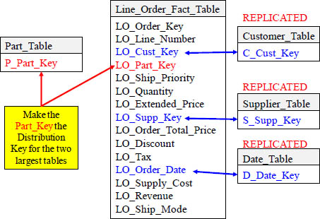
The fact table (Line_Order_Fact_Table) is the largest table, but the Part_Table is the largest dimension table. That is why you make Part_Key the distribution key for both tables. Now, when these two tables are joined together, the matching Part_Key rows are on the same Node. You can then distribute by UNSEGMENTED, which replicates the other dimension tables to each node. Each table will have all their rows on each Node. Now, everything that joins to the fact table is co-located!

Why a Sort Key Improves Performance

There are three basic reasons to use the sortkey keyword when creating a table. 1) If recent data is queried most frequently, specify the timestamp or date column as the leading column for the sort key. 2) If you do frequent range filtering or equality filtering on one column, specify that column as the sort key. 3) If you frequently join a (dimension) table, specify the join column as the sort key. Above, you can see we have made our sortkey the Order_Date column. Look how the data is sorted!

Sort Keys Help Group By, Order By and Window Functions

When data is sorted on a strategic column, it will improve (GROUP BY and ORDER BY operations), window functions (PARTITION BY and ORDER BY operations), and even as a means of optimizing compression. But, as new rows are incrementally loaded, these new rows are sorted but they reside temporarily in a separate region on disk. In order to maintain a fully sorted table, you need to run the VACUUM command at regular intervals. You will also need to run ANALYZE.