18
All Perovskite Tandem Solar Cells
Zhaoning Song and Yanfa Yan
The University of Toledo, Wright Center for Photovoltaics Innovation and Commercialization, Department of Physics and Astronomy, 2801 W. Bancroft St., Toledo, OH, 43606, USA
18.1 Introduction
In recent years, organic–inorganic metal halide perovskite solar cells (PSCs) have emerged as a promising photovoltaic (PV) technology, extending the frontiers of research and development in renewable energy generation [1]. The unprecedented rapid development of PSCs has attracted tremendous academic and industrial interest and extensive research efforts [2]. Within a decade, the power conversion efficiency (PCE) of single‐junction solar cells has climbed from 3.8% [3] to a certified 25.2% [4]. As the PCE record of PSCs is quickly approaching the thermodynamical efficiency limits (∼33%) of single‐junction cells set by the Shockley–Queisser (S–Q) detailed balance theory [5], the strategies to develop the next‐generation PSCs that have a potential to surpass such an efficiency ceiling have been proposed and studied. So far, the only PV technology that has demonstrated such potential is multijunction tandem solar cells [6]. Notably, the metal halide perovskite materials are an ideal candidate for fabricating tandem solar cells [7–10], due to their bandgap tunability in a wide range from 1.1 to ∼3 eV [11], low‐temperature (less than 150 °C) solution‐based processing methods [12–14], and low estimated manufacturing costs of ∼US$ 0.4 per peak watt [15, 16].
Tandem solar cells combining a wide‐bandgap (1.6–1.9 eV) perovskite top cell and a low‐bandgap (1.1–1.3 eV) bottom cell, such as mixed tin (Sn)‐lead (Pb) perovskite, crystalline silicon (Si), or copper indium gallium selenide (CIGS), offer an extraordinary opportunity to achieve PCEs higher than S–Q limit for single‐junction solar cells [7–10]. Among various perovskite tandem configurations, all‐perovskite tandem solar cells (APTSCs) consisting of two perovskite subcells with complementary bandgaps possess unique advantages [10], including low‐temperature processes for all subcells [17], compatibility with flexible and lightweight applications [18], low life‐cycle environmental impacts and embodied energy [19–21], and potentially low fabrication costs [22, 23]. To date, APTSCs with two‐terminal (2‐T) and four‐terminal (4‐T) tandem configurations have demonstrated PCEs of up to 24.8% [24] and 25% [25], close to the record PCE of single‐junction PSCs. Such tandem combinations hold a promise to achieve theoretical maximum PCEs of more than 40% [7, 26].
One of the distinct advantages of metal halide perovskite materials that enable the fabrication of APTSCs is bandgap tunability via adjusting the stoichiometry of perovskites. A common metal halide perovskite can be described by a formula ABX3, where A, B, and X represent a monovalent cation (e.g. methylammonium (MA)+, formamidinium (FA)+, Cs+, and Rb+), a divalent cation (e.g. Pb2+, Sn2+, Ge2+), and a halogen anion (e.g. I−, Br−, and Cl−), respectively. The crystal structure is constructed by a framework of corner‐sharing metal halide (BX3−) octahedra with the voids filling by monovalent cations A+, as depicted in Figure 18.1a. Methylammonium lead iodide (MAPbI3) with a bandgap of ∼1.55 eV is the prototypical and most widely used compound [27]. Substituting A, B, and X sites with different elements can tune the optical absorption band edge in the range of ∼400 to 1100 nm, corresponding to a bandgap range of 3.1 to ∼1.1 eV, as shown in Figure 18.1b. The wide‐bandgap (>1.7 eV) perovskites are typically synthesized with halide substitution using smaller‐sized anions. For example, substituting I− with Br− and Cl− shifts the bandgap of MAPbX3 from 1.6 (MAPbI3) to 2.3 (MAPbBr3) and 3.1 eV (MAPbCl3), respectively [28, 29]. The low‐bandgap (1.1–1.3 eV) perovskites are achieved by intermixing of Sn‐ and Pb‐based iodide perovskites, which allows narrowing of bandgap to the near‐infrared (NIR) range of ∼1.1 eV with approximately 50% Sn substitution [30–32]. This wide range of bandgap tunability, covering from NIR to ultraviolet (UV), allows the combination of two complementary bandgaps of perovskites, which utilizes the solar spectrum more efficiently than a single bandgap absorber, enabling the applications of APTSCs.
In this chapter, we will review the theory and major advancements of APTSCs in recent years. We first discuss the working principles of tandem solar cells. After that, recent progress and issues in wide‐ and low‐bandgap single‐junction PSCs are summarized. We then provide a survey of current state‐of‐the‐art APTSCs and discuss the limitations and challenges for APTSCs. Lastly, we conclude with an outlook for the future development of APTSCs.

Figure 18.1 (a) Crystal structure of an ABX3 perovskite and representative elements. (b) Band gap ranges for ABX3 perovskites with different combinations of elements.
18.2 Working Principles of Tandem Solar Cells
18.2.1 Why to Use Tandem Solar Cells
Figure 18.2a plots the maximum achievable PCE for a single‐junction solar cell governed by the bandgap (Eg) of the absorber material, which is known as the S–Q limit [5]. Limited by the intrinsic thermodynamic energy loss, a bandgap value in the range of 1.1–1.4 eV is optimal for achieving the maximum PCE values of ∼33%. Figure 18.2b illustrates a simple graphic analysis of intrinsic energy losses in a single‐junction solar cell [33], including optical (no absorption) and thermal (thermalization) losses. In brief, photons with energies lower than the bandgap of a semiconductor absorber (hυ < Eg) cannot be absorbed, whereas photons with energies higher than the absorber bandgap (hυ > Eg) excite electron–hole pairs to higher energy states and then lose the excess energy above the bandgap by releasing heat (Figure 18.2c). As a result, an absorber material with a narrower bandgap is desired to harvest more photons but suffers more severely from the thermalization loss of high‐energy photons. This trade‐off between the optical and thermal losses determines the theoretical limit of a solar cell with an absorber layer.
Multijunction tandem solar cells have been proved to be an effective approach to break the thermodynamic efficiency limit of single‐junction cells. The purpose of utilizing multiple absorber layers with different bandgaps is to mitigate intrinsic energy losses from the thermalization of photoexcited carriers [10]. For example, a double‐junction tandem solar cell consisting of two absorber materials with complementary bandgaps can utilize the whole solar spectrum effectively (Figure 18.2d). A top cell with a wider bandgap is used to harvest high‐energy photons, while a bottom cell with a lower bandgap is used to absorb low‐energy photons that penetrate deeper into the bottom cell. This tandem combination ensures the maximum harvest of the full solar spectrum with lower intrinsic thermalization losses than a single‐junction solar cell and therefore, holds a promise to achieve higher PCEs than the S–Q limit of single‐junction cells. Similar to the single‐junction device, there exist thermodynamic limits for the double‐junction tandem solar cells [26], which are determined by the combination of bandgap values of the top and bottom cells and the constraints on subcell integration. Using multijunction (more than two junctions) tandem configurations can further raise the efficiency ceiling from ∼46% for double junction to more than 60% for septuple and octuple junction (Figure 18.2e) [34]. So far, the highest PCE exceeding 50% has been demonstrated by sextuple‐junction III–V tandem cells [35]. Despite the promising for ultrahigh PCE, it is challenging to fabricate multijunction tandem solar cell devices due to processing and structural complexity. Moreover, in practice, the potential efficiency gains typically are insufficient to compensate for the additional processing time and costs. Therefore, for the low‐cost and high‐efficiency terrestrial PV applications, double‐junction tandem configurations are commonly considered for perovskite‐based tandem solar cells.

Figure 18.2 (a) Thermodynamic S–Q efficiency limit for single‐junction solar cells. (b) Graphical analysis and (c) schematic illustration of primary sources of energy losses in a single‐junction solar cell. (d) AM1.5 solar spectrum and spectrum utilization of a double‐junction tandem solar cell. (e) Efficiency limit for multijunction tandem solar cells connected in series.
Source: (c) and (d) Song et al. [10].
18.2.2 Tandem Device Architectures
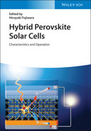
Double‐junction tandem solar cells are typically categorized based on the number of external terminals in a tandem device. A 4‐T tandem device comprises two separate solar cells, each with two independent external electrodes. The two cells can be typically assembled into a tandem system by mechanically stacking (Figure 18.3a). The back electrode of the top cell is usually transparent, allowing long‐wavelength photons to penetrate the top cell and enter the bottom one. Alternatively, an optical splitter can be used to divide the solar spectrum into two parts and distribute the light to individual solar cells (Figure 18.3b). For practical use, the mechanically stacked 4‐T configuration is more widely adopted than the optical‐splitting one due to its simplicity. Figure 18.3c shows a schematic structure of a 2‐T tandem solar cell, consisting of two subcells fabricated on the same substrate and monolithically integrated. A 2‐T tandem device has two external electrodes: a transparent front electrode and an opaque back electrode. The two subcells are connected internally by an interconnecting layer (ICL). Different tandem configurations have their pros and cons. For instance, 4‐T tandem cells possess design and fabrication simplicity but require more materials (extra substrate and transparent electrodes) and more balance of system components (frames, wires, invertors, etc.) to support the operation of solar panels. In contrast, 2‐T tandem cells are fabricated monolithically in a concise device architecture but have unique challenges in the design and device fabrication.
The subcells of a tandem solar cell can be regarded as individual single‐junction solar cells. High‐efficiency single‐junction PSCs are fabricated in the so‐called n‐i‐p and p‐i‐n device structures, as shown in Figure 18.4. The naming convention of PSCs represents the sequence of device preparation. Since most PSCs are in the superstrate configuration, i.e. light incident from the glass substrate, the fabrication sequence is the same as the light propagation direction. For the n‐i‐p structure (Figure 18.4a), a film stack consisting of a transparent conductive oxide (TCO) front electrode, an n‐type electron selective layer (ESL), a perovskite absorber layer, a p‐type hole selective layer (HSL), and a back electrode is sequentially deposited on a glass substrate. For the p‐i‐n structure, the sequences of ESL and HSL are exchanged (Figure 18.4b). High‐efficiency wide‐bandgap PSCs are made in both configurations. Low‐bandgap PSCs, however, are mostly made in the p‐i‐n configurations.
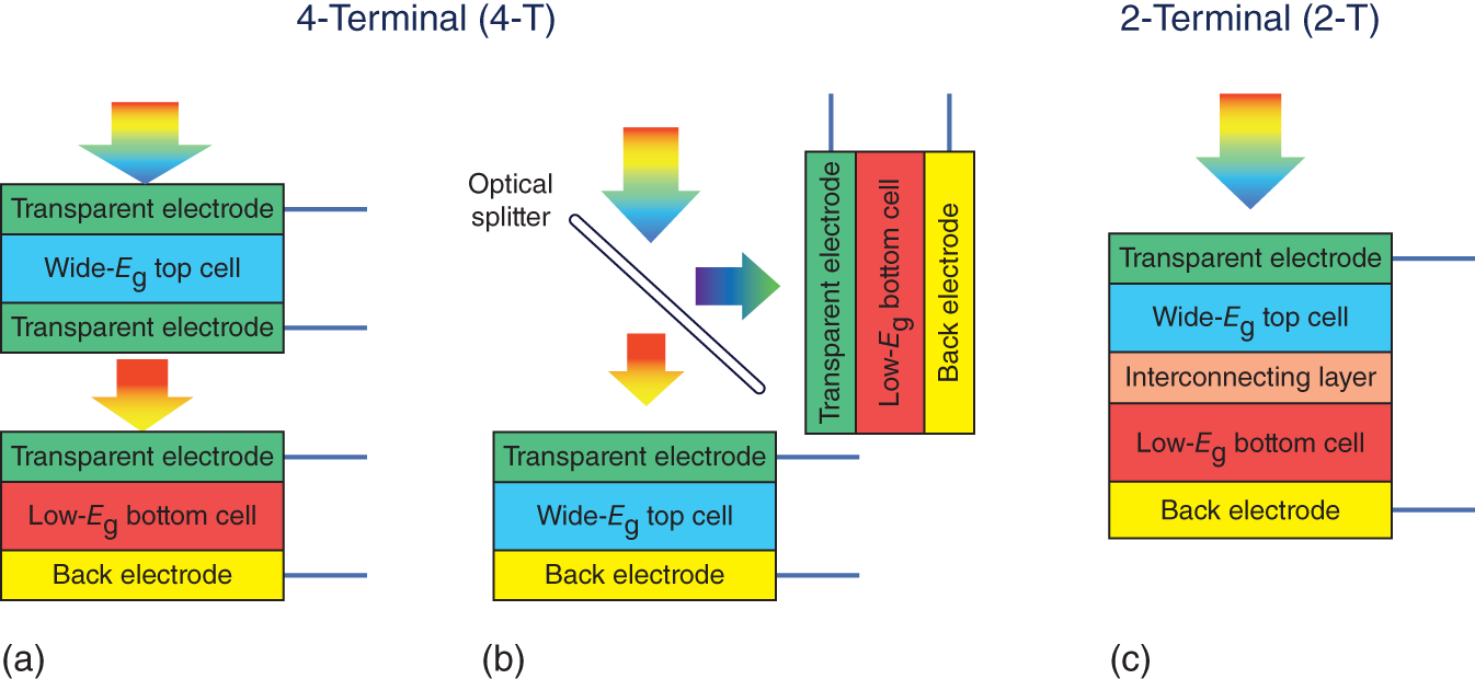
Figure 18.3 Schematic illustration of (a) 4‐T mechanically stacked, (b) 4‐T optically splitting, and (c) 2‐T monolithically integrated tandem solar cells.
Source: Song et al. [10].
Figure 18.4 General device structures of perovskite solar cells with (a) n‐i‐p and (b) p‐i‐n device configurations.
Source: Song et al. [10].
18.2.3 PCE of Tandem Solar Cells
The operation principles of 4‐T and 2‐T tandem solar cells are different. Figure 18.5 plots the J–V curves of 4‐T and 2‐T tandem solar cells and their corresponding subcells. For a 4‐T tandem solar cell, the two subcells are optically coupled but not electronically connected. A 4‐T tandem solar cell is not a single working device but two individual cells operating separately at the same time (Figure 18.5a). Typically, the total PCE of a 4‐T tandem device can be calculated by summing up the PCEs of individual subcells, as to express in Eqs. (18.1)–(18.3):
where ηtandem, ηtop, and ηbottom are PCEs for tandem, top, and bottom cells, respectively; VOC, top, VOC, bottom, JSC, top, JSC, bottom, FFtop, and FFbottom are open‐circuit voltage (VOC), short‐circuit current density (JSC), and fill factor (FF) of the top and bottom subcells, respectively. Because the total tandem PCE is just a mathematical sum of two subcells, 4‐T tandem solar cells are also referred as unconstraint tandem solar cells.
For a 2‐T tandem solar cell, the two subcells are electrically connected in series. Therefore, current and voltage behaviors of the system follow the Kirchhoff's law, i.e. the voltage of tandem is the sum of that of two subcells, whereas the current is the same for the whole device (Figure 18.5b). Note that a 2‐T tandem solar cell generally outputs only one J–V curve that represents the performance of the whole device. The J–V curves of corresponding subcells are only used for device analysis and cannot be directly measured. The total PCE of a 2‐T tandem is governed by Eqs. (18.4)–(18.6):

Figure 18.5 Simulated J–V curves of (a) two subcells in a 4‐T tandem cell and (b) a 2‐T tandem cell and its subcells.
where Vtandem, Vtop, Vbottom, Jtandem, Jtop, and Jbottom, are voltage and current density of tandem, top, and bottom cells, respectively. Because of the current match condition, 2‐T tandem solar cells are also named as constraint tandem solar cells.
Figure 18.6 plots the theoretical limits of PCEs of 2‐T and 4‐T tandem solar cells with respect to the bandgap energies of top and bottom cells. For 4‐T tandem cells, because the subcells operate individually, there is no constraint on the selection of bandgaps. As a result, the PCE limit of 4‐T tandem cells is not very sensitive to the variation in bandgap (Figure 18.6a). PCEs of more than 40% are achievable for a wide range of bandgap combinations. For monolithic 2‐T tandem cells, the series connection requires both subcells to generate identical current. This current match condition presents constraints on the design of absorber bandgap and thickness, limiting the optimal bandgap combination to a narrower attainable range (Figure 18.6b). For APTSC applications with a bottom cell bandgap of ∼1.2 eV, both 4‐T and 2‐T configurations have the potential to reach PCEs over 40%.

Figure 18.6 Theoretical efficiency limits of (a) 4‐T and (b) 2‐T tandem solar cells.
In real‐world applications, the design of tandem solar cells also needs to consider the spectrum variation from the standard measurement conditions. Geographic factors, such as attitude, irradiance, temperature, and humidity, may influence the annual energy yield of tandem solar cells [36–39]. A recent study compared the energy yield at different locations and concluded that matching bandgap pairs exactly at the maximum PCE points are not essential for the fabrication of high‐performance perovskite tandem solar cells [36]. This result shows some tolerances on the compositional control during the preparation of perovskite absorber layers for tandem solar cells. Therefore, a variety of bandgap combinations developed in the laboratory can be used for the fabrication of perovskite tandem solar cells.
18.3 Wide‐Bandgap Perovskite Solar Cells
18.3.1 Wide‐Bandgap Mixed I‐Br Perovskites
APTSCs use wide‐bandgap perovskite subcells to minimize the thermalization loss of high‐energy photons. A high‐efficiency wide‐bandgap PSC is essential to maximize the voltage and performance of a tandem device. To achieve high‐performance APTSCs, it is critical to judiciously select the bandgap of the top cell. According to the theoretical PCE calculation shown in Figure 18.6, a top cell bandgap in the range of 1.65–1.85 eV is desired to pair with low‐bandgap mixed Sn‐Pb perovskite (Eg = ∼1.2 eV). This bandgap range is readily accessible for mixed halide perovskites by partially substituting Br for I in iodide‐based perovskites (Figure 18.7). Increasing the Br proportion typically increases the bandgap of perovskite. Noh et al. [28] and Eperon et al. [40] investigated the bandgap tunability of single‐monovalent‐cation perovskites, MAPb(I1–xBrx)3 and FAPb(I1–xBrx)3, respectively. They demonstrated that the bandgap of mixed halide perovskites could be tuned in a wide range from 1.5 to 2.3 eV. Beal et al. investigated inorganic CsPb(I1–xBrx)3 perovskites, showing a tunable bandgap range of 1.8–2.3 eV [41]. Although these mixed I‐Br perovskites show continuously tunable bandgap range, for perovskites with a relatively high Br proportion (>30 mol%), it is challenging to maintain their bandgap energy and deliver the expected high VOC values in corresponding devices. This VOC loss is mainly attributed to photoinduced halide phase segregation and a high density of defects in the mixed halide perovskites [42].
The commonly used absorber compositions for efficient wide‐bandgap PSCs can be described as APb(BrxI1–x)3, where A is a combination of MA, FA, and Cs. The bandgap is typically adjusted by tuning the halide ratio. Br molar ratios of 20–40% are typically used for wide‐bandgap PSCs. The ternary combination space of monovalent cations (Cs, FA, MA) and the corresponding PCEs for wide‐bandgap PSCs reported in the literature are summarized in Figure 18.8a. The bandgap values of the mostly used wide‐bandgap perovskites as a function of the Br proportion are depicted in Figure 18.8b. It is worth noting that various bandgap values have been reported for mixed I‐Br perovskites with the same Br proportions because the methods to determine the bandgap are different. For a straightforward comparison, it is proposed that a unique and easily applicable approach should be used as a general reference [43]. It can be seen in Figure 18.8 that the most commonly used absorbers for wide‐bandgap PSCs are FA‐based (FA > 75 mol%) perovskites with small proportions of Cs and/or MA (MA + Cs < 25%) to stabilize the perovskite phase and with Br proportions of 20–40%. These compositions were selected from a complicated compositional space for fabricating efficient and stable wide‐bandgap PSCs.

Figure 18.7 Bandgap variations of mixed I‐Br perovskites. Bandgap values of MA, FA, Cs‐based mixed I‐Br perovskites are adapted from Refs. [28, 40, 41], respectively.
Sources: Adapted from Noh et al. [28]; Eperon et al. [40]; and Beal et al. [41].

Figure 18.8 (a) Ternary monovalent cation composition of wide‐bandgap mixed I‐Br perovskites and the PCEs for corresponding PV devices. (b) Bandgap as a function of Sn proportion for commonly used wide‐bandgap mixed I‐Br perovskites and the PCEs for corresponding PV devices.
It is worth noting that wide‐bandgap PSCs typically exhibit high VOC‐deficits, defined as Eg/e–VOC, where e is the unit charge. Hoke et al. found the reversible photoinduced trap formation in mixed halide hybrid perovskites [44]. They showed that the high Br content in MAPb(I1–xBrx)3 films caused the intense subbandgap photoemission, which is detrimental to the device performance. The photoinstability of mixed halide perovskite is later known as the halide phase segregation [45, 46], which is the primary limitation that causes the VOC‐deficits and greatly limited the progress of wide‐bandgap PSCs. Many research efforts have been paid to overcoming the phase segregation of the mixed halide perovskites. Among them, McMeekin et al. demonstrated a series of efficient wide‐bandgap PSCs with FA/Cs‐based mixed cation perovskites [47]. The FA/Cs‐based perovskites exhibit better phase stability than the pure MA‐ or FA‐based perovskites under heat and light. Due to the excellent phase stability and device performance, the CsyFA1–yPb(I1–xBrx)3 perovskite is now one of the most popular choices for the wide‐bandgap PSCs.
18.3.2 Current State of Wide‐Bandgap Perovskite Solar Cells
High‐efficiency wide‐bandgap PSCs are fabricated in both n‐i‐p and p‐i‐n device configurations. The n‐i‐p device architecture typically consists of an indium tin oxide (ITO) or fluorine‐doped tin oxide (FTO)‐coated glass substrate, an SnO2 or TiO2 ESL, a wide‐bandgap mixed I‐Br perovskite absorber layer, a 2,2′,7,7′‐Tetrakis[N,N‐di(4‐methoxyphenyl)amino]‐9,9′‐spirobifluorene (Spiro‐OMeTAD) HSL, and a gold (Au) back electrode (Figure 18.9a). The p‐i‐n device architecture typically consists of an ITO‐coated glass substrate, a poly[bis(4‐phenyl)(2,4,6‐trimethylphenyl)amine] (PTAA) HSL, a wide‐bandgap mixed I‐Br perovskite absorber layer, a fullerene‐based ESL (e.g. C60 or [6,6]‐Phenyl C61 butyric acid methyl ester [PCBM]), a bathocuproine (BCP) hole‐blocking layer, and a silver (Ag) back electrode (Figure 18.9b). When wide‐bandgap PSCs are used for the top cell in a tandem application, the back electrode is replaced by a TCO layer, e.g. ITO [48] or indium‐doped zinc oxide (IZO) [49].
Currently, the state‐of‐the‐art wide‐bandgap PSCs with absorber bandgaps of more than 1.7 eV are mainly based on Cs/FA perovskites with proper bulk and surface passivation. Tan et al. modified FA/Cs‐based mixed cation perovskites by introducing dipolar cations (MA), which healed the deep traps in wide‐bandgap perovskites [50]. They fabricated wide‐bandgap PSCs in the n‐i‐p structure using Cs0.12MA0.05FA0.83Pb(I0.6Br0.4)3 absorber layers with a bandgap of 1.74‐eV, demonstrating a high PCE of 19.1% with a high VOC of 1.25 V. Gharibzadeh et al. passivated the top surface of Cs0.17FA0.83Pb(I0.6Br0.4)3 perovskite (Eg = 1.72 eV) with butylammonium bromide (BABr) [51]. Their champion device with the n‐i‐p structure exhibited a PCE of 19.4%, with a remarkably high VOC of 1.31 V.

Figure 18.9 Most common material selection for wide‐bandgap PSCs in (a) n‐i‐p and (b) p‐i‐n device configurations.
The wide‐bandgap PSCs in the p‐i‐n structure currently exhibit inferior performance than the n‐i‐p counterparts, likely due to interface recombination/band misalignment at the perovskite/ESL interface. Strategies have been developed to mitigate the charge extraction at the ESL interface. Lin et al. fabricated 1.71‐eV p‐i‐n type wide‐bandgap PSCs with (FA0.83MA0.17)0.95Cs0.05Pb(I0.6Br0.4)3 absorber layers [52]. An isolating isomer of indene‐C60 bisadduct (ICBA‐trans3) ESL was used to tune energy level alignment with wide‐bandgap perovskites, resulting in a PCE of 18.5% with a VOC of 1.21 V. Chen et al. used guanidinium bromide (GABr) to from a 2D/3D graded homojunction interface on the mixed halide perovskite films. The best device demonstrated a PCE of 18.1% with a high VOC of 1.24 V [53]. It is worth noting that current 2‐T APTSC requires a p‐i‐n type device configuration due to the limitation of low‐bandgap PSCs. Therefore, there is a great need to further improve the performance of p‐i‐n wide‐bandgap PSCs. Palmstrom et al. incorporated dimethylammonium (DMA) into perovskite composition to form FA0.6Cs0.3DMA0.1PbI2.4Br0.6 with a bandgap of 1.7 eV, demonstrating a PCE of 19.2% for the champion device [39].
18.3.3 Critical Issues of Wide‐Bandgap Perovskite Cells
One of the most significant shortcomings and limitations of current wide‐bandgap PSCs is the relatively large VOC‐deficits, consequently leading to inferior PCEs. Figure 18.10 shows the VOC and PCE values of representative wide‐bandgap PSCs reported in the literature. Despite the rapid progress in recent years, most wide‐bandgap PSCs still exhibit VOC‐deficits in the order of 0.5 V with only one exception of ∼0.4 V [51] (Figure 18.10a). Such VOC‐deficits are higher than their lower bandgap counterparts, which typically have VOC‐deficits as low as 0.3 V [54]. For the desired bandgap range (1.7–1.9 eV) for APTSCs, a higher VOC can hardly be realized by increasing the perovskite bandgap due to the increasing VOC‐deficit. As a result, wide‐bandgap PSCs with a higher bandgap typically exhibit a lower PCE, as shown in Figure 18.10b. The VOC limitation presents a critical challenge for further improving the performance of APTSCs.
The large VOC‐deficit in wide‐bandgap PSCs is mainly attributed to the intrinsic photoinduced phase segregation [55–58]. Under illumination, the compositionally uniform mixed I‐Br perovskite alloy tends to segregate into a mixture of I‐rich and Br‐rich domains. The I‐rich domains trap photoexcited charge carriers, limiting the quasi‐Fermi energy splitting, and therefore, limiting the photovoltage generated in the perovskite absorber layer. Additionally, phase segregation and halide migration under electric field also degrade the device performance of wide‐bandgap PSCs [45, 59–63].

Figure 18.10 Reported (a) VOC and (b) PCE of wide‐bandgap PSCs as a function of absorber bandgap.
Source: Song et al. [10].
In recent years, a variety of strategies have been developed to mitigate the phase segregation in mixed I‐Br wide‐bandgap perovskites and hence improve the PCE. Some success has been achieved, including the modification of perovskite stoichiometry (e.g. high Cs+ proportion [64] and Sn2+ incorporation [65]), grain boundary passivation using potassium (K+) [66], perovskite surface passivation [67], improvement in crystallinity and grain sizes of perovskite films [68], synthesis of size‐tuned nanocrystals [69], and formation of 2D/3D perovskites [70–72]. Among these strategies, the 2D/3D perovskite bulk and surface passivation are the most effective one. For instance, Xiao et al. incorporated n‐butylammonium iodide (BAI) into mixed halide perovskites to form a self‐assembled capping layer to stabilize bandgaps of perovskites [71]. Stoddard et al. showed enhanced defect tolerance and phase stability of wide‐bandgap perovskite films via guanidinium (GA) alloying [70]. Rajagopal et al. incorporated small amounts of phenylethylammonium (PEA) cations in MAPb(I0.6Br0.4) perovskites, improving the VOC of wide‐bandgap PSCs to 1.35 V [72].
Despite the aforementioned approaches to enhance the phase stability and performance of wide‐bandgap mixed I‐Br perovskite films and devices, there still needs a way to address the phase instability issue. To achieve this goal, the entire ABX3 stoichiometric space, including all the possible 2D/3D combinations, needs to be systematically explored. This may need to rely on machine learning [73] and automatic high‐throughput robots [74] to synthesize and evaluate the phase stability of newly developed wide‐bandgap perovskite films.
18.4 Low‐Bandgap Perovskite Solar Cells
18.4.1 Low‐Bandgap Mixed Sn‐Pb Perovskites
High‐performance APTSCs require high‐efficiency and stable low‐bandgap perovskites. Low‐bandgap perovskites with a bandgap of ∼1.1 to 1.3 eV are typically synthesized by partially substituting Pb by Sn in the Pb‐iodide perovskites. Mixed Sn‐Pb perovskites possess some unique optoelectronic properties, such as the bandgap bowing effect [75] and high intrinsic carrier concentrations [30]. Additionally, low‐bandgap mixed Sn‐Pb perovskites suffer from the instability issue due to the ease of oxidation of Sn2+ to Sn4+, resulting in much‐shortened device durability and poor operational stability compared with their wider bandgap (>1.4 eV) Pb‐based counterparts.
A variety of compositions have been developed for the mixed Sn‐Pb perovskites. The commonly used cation combinations (FA, MA, and Cs) and the best reported PCE of the corresponding PSCs are shown in Figure 18.11. The best‐performing compositions are based on FA/MA mixed stoichiometry with MA proportion of 30–50% and Sn proportion of 50–60%. This compositional space was rationally selected as a result of extensive research efforts over the past few years.
In 2014, Hayase and coworkers found that MASnxPb1–xI3 perovskites synthesized by mixing MASnI3 and MAPbI3 exhibited bandgap values as low as 1.17 eV, lower than that of both MASnI3 (∼1.35 eV) and MAPbI3 (1.55 eV) [76]. Kanatzidis group then systematically investigated the structural and optical properties of MASnxPb1–xI3 perovskites, revealing an anomalous bandgap bowing effect in the mixed Sn‐Pb perovskites (Figure 18.12) [31, 75]. The origins of the bandgap bowing have been attributed to the spin–orbit coupling (SOC) and the lattice distortion [75] and mismatched band edges formed by Pb‐p and I‐p/Sn‐s [80, 81]. The bandgap bowing effect has also been shown in mixed Sn‐Pb perovskites with other monovalent cations (FA and Cs) (Figure 18.12) [77, 78].
Among various mixed Sn‐Pb perovskites, mixed organic cation (MA/FA) low‐bandgap perovskites exhibit the best device performance. In 2016, Yang et al. explored mixed cation MA1–xFAxPb0.75Sn0.25I3 perovskites for low‐bandgap PSC applications. Their champion devices based on 1.33‐eV MA0.5FA0.5Pb0.75Sn0.25I3 PSCs exhibited a PCE of 14.2% [82]. Yan and coworkers developed a single‐step spin‐coating method to synthesize (FASnI3)1–x(MAPbI3)x perovskites by combining FASnI3 and MAPbI3 precursor solutions (Figure 18.13a) [79]. The best‐performing devices (PCE = 15%) were fabricated using (FASnI3)0.6(MAPbI3)0.4 perovskite with a bandgap of 1.25 eV. By increasing the concentration of the mixed precursor solution, perovskite grain sizes were increased to 1 μm, and the thickness of the mixed Sn‐Pb absorber was increased to more than 600 nm (Figure 18.13b) [83]. The thicker perovskite films exhibited longer carrier lifetimes of up to ∼250 ns (Figure 18.13c), allowing more efficient collection of photoexcited minority charge carriers. The PSCs with thicker absorber layers showed higher absorption of NIR photons, resulting in higher external quantum efficiencies (EQEs) in the long wavelength region (750–1000 nm) (Figure 18.13d). The best‐performing device exhibited a certified PCE of ∼17% (Figure 18.13e). Yan and coworkers further demonstrated that bulk and grain boundary passivation of (FASnI3)0.6(MAPbI3)0.4 perovskite via halide (Cl and Br) incorporation led to improved electronic properties and reduced recombination in the mixed Sn‐Pb PSCs, enabling high PCEs exceeding 19% [84, 85]. The desirable optoelectronic characteristics of (FASnI3)0.6(MAPbI3)0.4 were later confirmed by many groups. Using this perovskite composition, Prasanna et al. [86], Xu et al. [87], and Jiang et al. [88] independently demonstrated low‐bandgap PSCs with PCEs of 17.8, 18, and 20.7%, respectively.

Figure 18.11 (a) Ternary monovalent cation composition of low‐bandgap mixed Sn‐Pb perovskites and the PCEs for corresponding PV devices. (b) Bandgap as a function of Sn proportion for commonly used low‐bandgap mixed Sn‐Pb perovskites and the PCEs for corresponding PV devices.

Figure 18.12 Bandgap bowing effect of low‐bandgap mixed Sn‐Pb perovskites with different monovalent cations, including the MA [75], FA [77], Cs [78], MA/FA [79], and FA/Cs [78].
Sources: Im et al. [75]; Eperon et al. [77]; Rajagopal et al. [78]; Liao et al. [79].
Although FA/MA‐based mixed Sn‐Pb perovskites show decent PV performance, their photostability is greatly limited due to containing MA. MA cations are known unstable under illumination [89, 90]. As a thermally stable alternative, low‐bandgap mixed Sn‐Pb perovskites with FA/Cs‐based compositions, i.e. FA1–yCsySnxPb1–xI3, have been developed. Compared with FA/MA‐based mixed Sn‐Pb perovskites, FA/Cs‐based mixed Sn‐Pb perovskites show much better thermal‐ and photostability, resulting in more stable operation under maximum power point (MPP) tracking. In 2016, Eperon et al. fabricated 1.2‐eV low‐bandgap PSCs based on FA0.75Cs0.25Sn0.5Pb0.5I3 [77]. The best‐performing device exhibited a PCE of 14.8%, much higher than the PCE of 10.9% for the control device based on FASn0.5Pb0.5I3. Recently, Leijtens et al. raised the PCE to 15.6% after incorporating MACl and formic acid into the precursor solution [91]. Zong et al. systematically investigated the compositional space of (FAPbI3)1−x(CsSnI3)x [92]. The (FAPbI3)0.7(CsSnI3)0.3 perovskite with an ideal bandgap of ∼1.3 eV for a single‐junction PSCs was used as the absorber layer of low‐bandgap PSCs, achieving a PCE of up to 14.6%. They recently incorporated Lewis‐adduct additive SnF2–3FACl to the precursor solution, improving the PCE of (FAPbI3)0.7(CsSnI3)0.3 PSCs to 15.8% [93].

Figure 18.13 (a) Schematic illustration and top‐view SEM images of the synthesis of (FASnI3)1–x(MAPbI3)x perovskites by mixing FASnI3 and MAPbI3 precursor solutions.
Source: Liao et al. [79].
(b) Top‐view and cross‐sectional SEM images of a 650 nm perovskite film. (c) TRPL lifetimes of perovskite films with different thicknesses and (d) EQE curves of corresponding devices. (e) The J–V curves of the best‐performing device.
Source: (b)–(e) Zhao et al. [83].
18.4.2 Current State of Low‐Bandgap Perovskite Solar Cells
State‐of‐the‐art low‐bandgap PSCs are mainly fabricated in the p‐i‐n device configuration, consisting of an ITO‐coated glass substrate, a poly(3,4‐ethylenedioxythiophene) polystyrene sulfonate (PEDOT:PSS) HSL, a low‐bandgap mixed Sn‐Pb perovskite absorber layer, a C60/BCP ESL, and an Ag back electrode (Figure 18.14a). The n‐i‐p configuration similar to Pb‐based PSCs (Figure 18.14b) was explored in the early development of low‐bandgap mixed Sn‐Pb PSCs. However, the n‐i‐p device architecture has rarely been used since 2014 [94]. High‐efficiency low‐bandgap PSCs with high Sn proportion (>50%) in the n‐i‐p structure are yet to be demonstrated. The challenges of the lack of effective charge selective layers (both ESL and HSL) and intrinsic oxygen sensitivity of mixed Sn‐Pb perovskites currently limit the development of low‐bandgap n‐i‐p type PSCs.
The best‐performing low‐bandgap PSCs are all based on the FA/MA perovskite synthesized by the single‐step spin‐coating method developed by Yan and coworkers [79, 83]. Several groups demonstrated low‐bandgap PSCs with PCEs exceeding 20%. Most recently, Yang et al. incorporated Cd2+ additives into FA0.5MA0.45Cs0.05Pb0.5Sn0.5I3 to enhance the electron diffusion length, achieving a PCE of 20.3% for the best‐performing device [95]. Tong et al. used guanidinium thiocyanate (GASCN) to passivate the grain boundary of (FASnI3)0.6(MAPbI3)0.4 perovskite [25]. A long carrier lifetime of more than 1 μs was achieved, which enabled low‐bandgap PSCs with a PCE of 20.4%. Lin et al. introduced elemental Sn into the precursor solution to suppress Sn2+ oxidation in the precursor ink [24]. They fabricated low‐bandgap PSCs using FA0.7MA0.3Pb0.5Sn0.5I3 absorber layer, demonstrating a remarkably high PCE of 21.1%.

Figure 18.14 Most common material selection for low‐bandgap PSCs in (a) p‐i‐n and (b) n‐i‐p device configurations.
18.4.3 Critical Issues of Low‐Bandgap Perovskite Cells
Despite remarkable progress in recent years, there remain some critical issues of low‐bandgap PSCs and APTSCs. The performance of low‐bandgap mixed Sn‐Pb PSCs is inferior to their pure Pb perovskite counterparts, due to higher non‐radiative recombination losses in bulk and at the interfaces of the mixed Sn‐Pb perovskite films. Particularly, due to relatively low absorption coefficients, the thickness of mixed Sn‐Pb perovskite layer needs to be on the order of 1 μm. However, the relatively higher carrier and defect densities in mixed Sn‐Pb perovskite films than pure‐Pb perovskites make the minority carrier lifetime and diffusion length shorter than that in their pure‐Pb counterparts.
We surveyed the low‐bandgap mixed Sn‐Pb PSCs reported in the literature and plot their JSC and PCE values vs. the bandgap value in Figure 18.15. Photocurrent in low‐bandgap PSCs still shows a large gap from the expected JSC values from the S–Q limit. The highest reported JSC value of the low‐bandgap PSCs that is confirmed by the EQE measurements is 31.4 mA/cm2 [25], realizing 78.5% of its theoretical potential. In comparison, PSCs with wider bandgap values show high JSC values exceeding 92% of the corresponding S–Q limits [96, 97]. Unlike the obvious JSC loss in the mixed Sn‐Pb PSCs, the highest reported VOC value of 0.888 V for a 1.27‐eV perovskite accounts for almost 90% of the S–Q limit [85]. The EQE analysis shows that the photon‐to‐electron conversation efficiency is less than 85% for a most of the spectral range (Figure 18.16). Moreover, most mixed Sn‐Pb PSCs show a significant photocurrent collection drops at long wavelengths due to insufficient light absorption. Therefore, achieving an adequate conversion of NIR photons requires the use of thick low‐bandgap mixed Sn‐Pb perovskite absorber layers. However, when the thickness is increased to certain values, other PV parameters such as VOC and FF start to decrease due to the presence of a significant number of defects in the mixed Sn‐Pb perovskites, which lead to short carrier lifetimes and diffusion lengths [10]. Therefore, it is critical to passivate bulk and grain boundaries defects and improve the lifetimes and diffusion lengths in the mixed Sn‐Pb perovskites are needed.

Figure 18.15 Reported (a) JSC and (b) PCE of low‐bandgap PSCs as a function of absorber bandgap.
Source: Song et al. [10].

Figure 18.16 EQE spectra of state‐of‐the‐art low‐bandgap PSCs.
Source: Data from Lin et al. [24]; Tong et al. [25]; Zhao et al. [84]; and Yang et al. [95].
Another serious issue for low‐bandgap mixed Sn‐Pb PSCs is the lack of material and device stability, especially under the working conditions. The material instability is attributed to the ease of oxidation of Sn2+ to Sn4+, which rapidly deteriorates the optoelectronic properties of mixed Sn‐Pb perovskite films, leading to a high density of holes, a short minority carrier lifetime, and a short minority carrier diffusion length in the degraded mixed Sn‐Pb films [94]. Additionally, high‐efficiency mixed Sn‐Pb PSCs typically contain a high proportion of MA (>30 mol%), which caused significant photoinstability [89, 98]. The PSCs based on MA‐contained mixed Sn‐Pb perovskites show much more severe photoinduced decay than FA/Cs‐based devices under MPP measurements [91]. The ease of material degradation also limits the fabrication route and the design of low‐bandgap single‐junction PSCs and APTSCs. Currently, most high‐efficiency low‐bandgap PSCs have been fabricated in the p‐i‐n device architectures (Figure 18.14a) with PEDOT:PSS and C60/BCP as the HSL and ESL, respectively. For the n‐i‐p device structure (Figure 18.14b), the commonly used metal oxide ESLs (e.g. SnO2 and TiO2) and the doped HSLs (e.g. spiro‐OMeTAD) are likely to induce the degradation of the mixed Sn‐Pb perovskites, limiting the device performance.
In recent years, many efforts have been made to mitigate the stability of low‐bandgap mixed Sn‐Pb PSCs. The most successful strategies include the use of more stable HSL/ESL and encapsulation. Chi et al. demonstrated better thermal‐ and photostability of mixed Sn‐Pb PSCs based on FAPb0.75Sn0.25I3 absorber after replacing PEDOT:PSS HSL by NiOx [99]. Leijtens et al. demonstrated that mixed Sn‐Pb PSCs with an ITO capping electrode survived after a thermal stability test at 85 °C in the air for more than 300 hours [91]. More recently, Prasanna et al. eliminated the PEDOT:PSS HSL and demonstrated remarkable device stability for mixed Sn‐Pb PSCs [100]. Remarkably, the mixed Sn‐Pb PSCs retained 95% of their initial efficiencies after 1000 hours at 85 °C in air with no encapsulation and in a damp heat test (85 °C with 85% relative humidity) with encapsulation. Additionally, the mixed Sn‐Pb PSCs showed negligible decay after MPP tracking under 1 sun illumination for over 1000 hours.
Another effective approach to mitigate the instability issue is the incorporation of antioxidant agents. Jen and coworkers used ascorbic acid as an antioxidant agent in the mixed Sn/Pb PSCs, demonstrating enhanced device stability compared with the control devices processed with regular reducing additive SnF2 [101]. Additionally, they developed another approach of forming stable mixed Sn‐Pb perovskite by using a galvanic displacement reaction [102]. By incorporating elemental Sn to the Pb‐based perovskite precursor solutions, they demonstrated a PCE of 18.21% for (FAPb0.6Sn0.4I3)0.85(MAPb0.6Sn0.4Br3)0.15‐based PSCs. The encapsulated cells retained more than 90% of their initial efficiencies after the storage in ambient air at room temperature or 80 °C for 1000 or 120 hours, respectively. Lin et al. incorporated metallic Sn powders in the conventional mixed Sn‐Pb perovskite precursor solution to suppress Sn2+ oxidation and demonstrated better device performance and stability [24]. This method was later confirmed by Jiang et al. in their study [88].
18.5 All‐Perovskite Tandem Solar Cells
APTSCs possess unique advantages, including low‐temperature processes for all subcells, compatibility with flexible and lightweight applications, and potentially low fabrication and environmental costs [19, 20]. Though potentially promising, it is challenging to fabricate efficient APTSCs due to the lack of highly efficient wide‐ and low‐bandgap perovskite subcells and difficulty of monolithically integrating two perovskite subcells in the 2‐T tandem configuration. The recent progress has propelled the PCEs of 4‐T and 2‐T APTSCs to 25% [25] and 24.8% [24], respectively (Figure 18.17), approaching the record of Pb‐based single‐junction PSCs. Clearly, the fabrication of high‐efficiency and stable high‐ and low‐bandgap PSCs is critical for realizing the full potential of APTSCs.
18.5.1 4‐T All‐Perovskite Tandem Solar Cells
The potential of using perovskite materials with complementary bandgaps for tandem solar cell applications has been first explored in the 4‐T tandem configuration. In 2016, Li et al. demonstrated the proof‐of‐concept 4‐T APTSCs by pairing 2.3‐eV MAPbBr3 and 1.6‐eV MAPbI3 as the top and bottom cells [103], achieving a PCE of ∼9.5%. Yang et al. demonstrated the first 4‐T APTSC with a low‐bandgap subcell by combining a 1.55‐eV MAPbI3 top cell and a 1.33‐eV MA0.5FA0.5Pb0.75Sn0.25I3 bottom cell, achieving a high PCE of 19.1% [82]. A thin absorber layer thickness of the MAPbI3 was used to allow sufficient photons to enter the bottom cell. As a result, PCEs of 13.5% and 5.6% (Figure 18.18a), with JSC values of 16.7 and 9.1 mA/cm2, were obtained for the top and filtered bottom cells, respectively. Later, Eperon et al. constructed 4‐T tandem cells with a better absorber combination consisting of a 1.6‐eV FA0.83Cs0.17Pb(I0.83Br0.17)3 top cell and a 1.2‐eV FA0.75Cs0.25Sn0.5Pb0.5I3 bottom cell [77]. With processing optimization, they achieved PCEs of 15.8% and 4.5% for the top and filtered bottom cells, respectively, resulting in a PCE of 20.3% for the 4‐T tandem cells (Figure 18.18b) [91]. In early 2018, Zhao et al. further enhanced the record 4‐T APTSC efficiencies to 23.1% by combining a FA0.8Cs0.2Pb(I0.7Br0.3)3 top cell with a (FASnI3)0.6(MAPbI3)0.4 bottom cell (Figure 18.18c) [48]. It is noticeable that this was the first time APTSCs demonstrated a PCE higher than the then‐record PCE (22.7%) of single‐junction PSCs (Figure 18.17). The incorporation of paraffin oil as an optical coupling layer between the two subcells reduces the optical loss at the air/glass interfaces, enabling PCEs of 15.7% and 7.4% for the top and flittered bottom cells, respectively. Most recently, Tong et al. paired a 1.63‐eV Cs0.05FA0.8MA0.15Pb(I0.85Br0.15)3 top cell with a 1.25‐eV GA‐passivated (FASnI3)0.6(MAPbI3)0.4 bottom cell to achieve a PCE of more than 25% (Figure 18.18d) [25]. This PCE was higher than the best‐performing single‐junction PSCs at the time, demonstrating a great potential of 4‐T APTSCs.

Figure 18.17 Evolution of PCEs for single‐junction PSCs and APTSCs.
Source: Song et al. [10].
18.5.2 2‐T All‐Perovskite Tandem Solar Cells
Compared with 4‐T tandem cells, 2‐T APTSCs are much difficult to design and fabricate. First, the interconnecting (IL) that integrates two subcells is a critical component in 2‐T APTSCs. The IL not only provides an optical and electrical interconnection between two subcells but also protects the underlying subcell from any damages introduced by processing the second cell. Second, to achieve the desired high PCE, the bandgap and thickness of absorber layers need to be finely adjusted to satisfy the current match condition. Finally, the complicated device architectures consisting of more than a dozen of layers are more prone to the processing flaws in each component layer, which will deteriorate the device performance and stability.

Figure 18.18 Replotted J–V curves of notable 4‐T APTSCs with various perovskite bandgap combination, including (a) 1.55‐eV/1.33‐eV.
Source: Based on Yang et al. [82], (b) 1.6‐eV/1.2‐eV.
Source: Based on Leijtens et al. [91], (c) 1.75‐eV/1.25‐eV.
Source: Based on Zhao et al. [48], and (d) 1.63‐eV/1.25‐eV.
Source: Based on Tong et al. [25].
Due to the lagged developed of low‐bandgap mixed Sn‐Pb PSCs, the early work on 2‐T APTSCs started with using 1.55‐eV MAPbI3 as the bottom cell. In 2015, Jiang et al. demonstrated the first proof‐of‐concept monolithic 2‐T APTSCs [104]. The tandem device comprises two MAPbI3 cells connected by organic ILs consisting of PEDOT:PSS/polyethylenimine (PEI)/PCBM:PEI (Figure 18.19a). Although the tandem device only exhibited a mediocre PCE of 7%, the high VOC value of 1.89 V was close to the sum of the two subcells, demonstrating the concept of 2‐T APTSCs. Meanwhile, Heo and Im fabricated 2‐T mechanically‐stacked APTSCs by physically laminating two separated subcells (MAPbBr3 and MAPbI3) together (Figure 18.19b) [105]. This stacked 2‐T tandem device delivered a PCE of 10.8% with a high VOC of 2.25 V. However, the JSC of this premature tandem device (8.3 mA/cm2) is limited by the relatively large bandgaps of the MAPbBr3 (2.2 eV) and MAPbI3 (1.55 eV) subcells and the physically contacted interconnecting interface. Bolink and coworkers constructed monolithic 2‐T APTSCs using solution‐processed wide‐bandgap FA0.75Cs0.25Pb(I0.3Br0.7)3 perovskite top cells, vacuum‐deposited MAPbI3 bottom cells, and doped/undoped organic ILs (Figure 18.19c). The champion tandem cell exhibited a PCE of 18.1%, with a high VOC of 2.14 V, a JSC of 9.7 mA/cm2, and an FF of 75.6% [106]. More recently, they also demonstrated all‐vacuum processed monolithic MAPbI3/MAPbI3 tandem cells, which yielded a PCE exceeding 18% with a remarkably high VOC of 2.30 V [107].
The first 2‐T monolithic APTSCs using a low‐bandgap mixed Sn‐Pb subcell was reported by Eperon et al. in 2016 [77]. The 2‐T tandem cells were constructed by combining a 1.8‐eV FA0.83Cs0.17Pb(I0.5Br0.5)3 top cell with a 1.2‐eV FA0.75Cs0.25Sn0.5Pb0.5I3 bottom cell using a zinc‐tin oxide (ZTO)/SnO2/ITO ILs (Figure 18.19d). The metal oxide ILs prepared by atomic layer deposition (ALD) and sputtering show decent optical and electrical properties and provide sufficient protection for processing the low‐bandgap mixed Sn‐Pb subcell. The rationally selected two subcells with complementary bandgaps (1.8/1.2 eV) allow broad absorption of the solar spectrum. The champion device delivered a PCE of 16.9%, with a VOC of 1.66 V, a JSC of 14.5 mA/cm2, and an FF of 70%. Leijtens et al. then adjusted the top cell composition to more photostable FA0.83Cs0.17Pb(I0.7Br0.3)3 and incorporated MACl and formic acid to improve the quality of the FA0.75Cs0.25Sn0.5Pb0.5I3 bottom cells, demonstrating APTSCs with a PCE of 19.1%, a VOC of 1.81 V, a JSC of 14.8 mA/cm2, and an FF of 71.3% [91]. Palmstrom et al. then improved the top cell by cation tuning (DMA and Cs), demonstrating PCEs of 23.1% and 21.3% for APTSCs built on rigid and flexible substrates [18] (Figure 18.20). This is the first and only time that flexible APTSCs have been reported.
Rajagopal et al. fabricated 2‐T APTSCs consisting of a 1.82‐eV MA0.9Cs0.1Pb(I0.6Br0.4)3 top cell and a 1.22‐eV MASn0.5Pb0.5I3 connected by a sputtered ITO recombination layer (Figure 18.19e), achieving a PCE of 18.4% [108]. Their 2‐T APTSCs demonstrated a high VOC of 1.98 V, which is approaching 80% of the theoretical voltage limit for this absorber combination. The tandem cell performance was limited by a relatively low JSC of ∼12.5 mA/cm2. Zhao et al. demonstrated efficient 2‐T APTSCs using a 1.75‐eV FA0.8Cs0.2Pb(I0.7Br0.3)3 top cell and a 1.25‐eV (FASnI3)0.6(MAPbI3)0.4 bottom cell connected by a simple vacuum‐processed MoO3/Ag/ITO ILs (Figure 18.19f) [84]. Chlorine was incorporated in the mixed Sn‐Pb perovskite to enlarge the grain size, increase carrier mobility, reduce electronic disorder, and suppress trap‐assisted recombination. The improved electronic quality led to the improved performance of low‐bandgap PSCs with an absorber layer thickness of ∼750 nm and enabled the fabrication of efficient 2‐T APTSCs. The best‐performing cells showed a VOC of 1.92 V, a JSC of 14.0 mA/cm2, and an FF of 78.1%, yielding a PCE of 21% [84]. The tandem cells showed decent operational stability, retaining over 85% of initial PCEs after 80 hours of continuous operation under MPP tracking conditions. Beyond the commonly used ITO‐based IL, Li et al. recently developed an ultrathin Cu/Au metal thermionic emission‐based IL for 2‐T APTSCs [109], demonstrating a new route to monolithically integrate two perovskite subcells.

Figure 18.19 (a)–(h) Various device structures developed for 2‐T APTSCs.
Efficiency breakthrough for 2‐T APTSCs was enabled by the fabrication of high‐quality 1‐μm‐thick mixed Sn‐Pb perovskite films in 2019. By combining GASCN‐passivated (FASnI3)0.6(MAPbI3)0.4 low‐bandgap cells with 1.75‐eV FA0.8Cs0.2Pb(I0.7Br0.3)3 top cells, Tong et al. reported monolithic 2‐T APTSCs with a PCE of 23.4%, a VOC of 1.942 V, a JSC of 15.01 mA/cm2, and an FF of 80.3% [25] (Figure 18.20). The operational stability of a 2‐T APTSC was monitored by MPP tracking under simulated one sun illumination. The tandem cell retained more than 88% of its initial efficiency after 100 hours of continuous operation. Yang et al. fabricated 2‐T APTSCs using 0.03% Cd2+‐incorporated Cs0.05MA0.45FA0.5Pb0.5Sn0.5I3 bottom cells and 1.8‐eV FA0.6Cs0.4Pb(I0.65Br0.35)3 top cells (Figure 18.19g) [95]. The best 2‐T tandem cell exhibited a PCE of 23.0%, with a VOC of 1.99 V, a JSC of 15.1 mA/cm2, and an FF of 77% (Figure 18.20). The device exhibited decent operational stability, retaining more than 90% of its initial PCE after 200 hours of operation. Lin et al. fabricated 2‐T APTSCs consisting of a 1.77‐eV FA0.8Cs0.2Pb(I0.6Br0.4)3 top cell and a 1.22‐eV FA0.7MA0.3Pb0.5Sn0.5I3 bottom cell connected by an ultrathin ALD SnO2/Au ILs (Figure 18.19h) [24]. The record efficiency 2‐T APTSC delivered a PCE of 24.8% under reverse scan, with a VOC of 1.965 V, a JSC of 15.6 mA/cm2, and a high FF of 81% (Figure 18.20). More importantly, the tandem cells retain 90% of their initial PCEs after more than 450 hours of continuous operation at the MPPs under one sun illumination.

Figure 18.20 J–V curves of notable 2‐T APTSCs.
Source: Data from Palmstrom et al. [18]; Lin et al. [24]; Tong et al. [25]; and Yang et al. [95].
18.5.3 Limitations and Challenges of All‐Perovskite Tandem Solar Cells
The recent research efforts in APTSCs have significantly advanced this promising PV technology. However, APTSCs are still in the premature stage of the development and far from commercial readiness. First, the scaling‐up fabrication presents a critical challenge for APTSCs. So far, most APTSCs reported in the literature have small active areas of less than 0.1 cm2, with only one exception with active areas of up to 1 cm2 [24]. These small device areas allow the commonly used spin‐coating processes to be applied for the fabrication of APTSCs. However, industrial manufacturing requires scaling‐up fabrication techniques for wide‐ and low‐bandgap PSCs and ILs. Moreover, the monolithic integration designs of APTSCs rely on the separation and interconnection of individual cells. The thin‐film tandem cell architecture designs and the methods for module integration are yet to be demonstrated. It is expected that more research efforts will be paid to the development in the design and fabrication of large‐area tandem cells and modules in the coming years.
Device reliability is another major concern for the applications of APTSCs. While APTSCs hold the promise to deliver high module efficiencies exceeding 30%, the requirement of robust lifetime of up to 25 years for commercial solar panels is a great challenge to overcome in their path toward commercialization. Although some promising stability testing results have been reported in the literature in recent years, the long‐term stability of PSCs is yet to be fully demonstrated. Especially for APTSCs, there are much smaller numbers of publications compared with reports of single‐junction PSCs. More importantly, standardized operational stability tests for APTSCs have rarely been reported. APTSCs are limited by the relatively poor stability of low‐bandgap mixed Sn‐Pb PSCs. Due to the vulnerability of mixed Sn‐Pb perovskites against oxygen and moisture, low‐bandgap mixed Sn‐Pb PSCs require complete encapsulation to work in the ambient conditions for a long time. Recently, MPP tracking of APTSCs under one sun illumination for up to hundreds of hours has been demonstrated by few groups [24, 25, 95]. Although such operational lifetime is not comparable with the single‐junction PSCs that have shown thousands of hours of MPP stability, these stability testing results are encouraging for further improvements of APTSCs. Nonetheless, stability issues of tandem PSCs need to be fully addressed before translating these promising PV technologies demonstrated in laboratories to real‐world applications [110].
Beyond the double‐junction APTSCs, multijunction tandem cells with more than two absorber materials will also be considered in the future development due to their potential to achieve higher theoretical limits. Werner et al. have demonstrated a high VOC of 2.69 V in a triple‐junction perovskite/perovskite/Si tandem cell [111]. McMeekin et al. fabricated the proof‐of‐concept triple‐junction APTSCs using a combination of 1.94 eV/1.57 eV/1.34 eV perovskites [17]. These attempts have opened up many new avenues for exploration of high‐efficiency low‐cost multijunction APTSCs. With more technology advances in the future, the full potential of multijunction APTSCs is expected to be realized.
18.6 Conclusion and Outlooks
The past decades have witnessed the rapid progress of metal halide perovskite PV technologies at an unprecedented speed. The success of Pb‐iodide single‐junction PSCs has propelled research advances in wide‐bandgap mixed I‐Br and low‐bandgap mixed Sn‐Pb PSCs, as well as high‐efficiency 2‐T and 4‐T APTSCs. Particularly, the recent breakthrough in high‐efficiency low‐bandgap mixed Sn‐Pb PSCs enabled the fabrication of 2‐T and 4‐T APTSCs with PCEs approaching the current record of single‐junction PSCs. Such a demonstration of high‐performance APTSCs is a long‐awaited sign showing the path of realizing the PCE potential of thin‐film tandem solar cells.
As the PCE of APTSCs is expected to further increase in the near future, the commercialization of this promising PV technology needs to be seriously considered. Future research efforts will be devoted to developing device architectures and deposition processes that are applicable for large‐area tandem perovskite PV module fabrication. The processing and environmental sensitivity of perovskite materials presents a major challenge for the design and fabrication of APTSCs. Particularly for the monolithically integrated 2‐T tandem cells, depositing the second perovskite subcells on the first‐prepared subcells requires special caution and protective remedies to mitigate the possible processing damages. This requires researchers to explore alternative tandem‐specific deposition approaches. One of the possible approaches is the vacuum‐based deposition [106, 107], which is not limited by the compactness of the top surface and solvent compatibility and can be adapted to the mild‐vacuum, low‐temperature, high‐throughput industrial production. The remaining challenges are how to achieve high‐quality perovskite films with different perovskite compositions, which require more research efforts.
Future work also needs to focus on developing more stable perovskite tandem modules. The desired device stability requires not only the advanced engineering on perovskite compositions and cell structures to enhance the stability of PSCs but also the module frame and encapsulation designs that prevent water and oxygen ingress [112–116] as well as the leakage of water‐soluble toxic Pb and Sn compounds [19, 117–119]. Once robust encapsulation can be implemented, APTSCs will have a chance to achieve sufficiently long‐term stability, which will benefit the adaption of these promising tandem techniques in the market. In the long future, APTSCs hold the potential to become the leader in the perovskite PV field due to their ultrahigh efficiency and low cost [120]. However, the route toward this ultimate promising perovskite PV technology is the most challenging one because of the performance and stability issues of the low‐bandgap PSCs. If these critical remaining issues can be resolved, APTSCs will fulfill their promise to deliver more electrical power at lower costs than today's PV technologies.
Acknowledgments
This material is based upon work supported by the U.S. Department of Energy's Office of Energy Efficiency and Renewable Energy (EERE) under the Solar Energy Technologies Office Award Number DE‐EE0008753. The U.S. Government is authorized to reproduce and distribute reprints for Governmental purposes notwithstanding any copyright notation thereon.
References
- 1 Correa‐Baena, J.‐P., Saliba, M., Buonassisi, T. et al. (2017). Science 358: 739–744.
- 2 Correa‐Baena, J.‐P., Abate, A., Saliba, M. et al. (2017). Energy Environ. Sci. 10: 710–727.
- 3 Kojima, A., Teshima, K., Shirai, Y., and Miyasaka, T. (2009). J. Am. Chem. Soc. 131: 6050–6051.
- 4 NREL Solar Cell Efficiency Chart. https://www.nrel.gov/pv/cell-efficiency.html (accessed 6 July 2019).
- 5 Shockley, W. and Queisser, H.J. (1961). J. Appl. Phys. 32: 510–519.
- 6 Green, M.A., Dunlop, E.D., Hohl‐Ebinger, J. et al. (2020). Prog. Photovolt. 28: 3–15.
- 7 Leijtens, T., Bush, K.A., Prasanna, R., and McGehee, M.D. (2018). Nat. Energy 3: 828–838.
- 8 Eperon, G.E., Hörantner, M.T., and Snaith, H.J. (2017). Nat. Rev. Chem. 1: 0095.
- 9 Anaya, M., Lozano, G., Calvo, M.E., and Míguez, H. (2017). Joule 1: 769–793.
- 10 Song, Z., Chen, C., Li, C. et al. (2019). Semicond. Sci. Technol. 34: 093001.
- 11 Saliba, M., Correa‐Baena, J.‐P., Grätzel, M. et al. (2018). Angew. Chem. Int. Ed. 57: 2554–2569.
- 12 Li, Z., Klein, T.R., Kim, D.H. et al. (2018). Nat. Rev. Mater. 3: 18017.
- 13 Song, Z., Watthage, S.C., Phillips, A.B., and Heben, M.J. (2016). J. Photon. Energy 6: 022001.
- 14 Yang, D., Yang, R., Priya, S., and Liu, S. (2019). Angew. Chem. Int. Ed. 58: 4466–4483.
- 15 Song, Z., McElvany, C.L., Phillips, A.B. et al. (2017). Energy Environ. Sci. 10: 1297–1305.
- 16 Chang, N.L., Ho‐Baillie, A.W.Y., Vak, D. et al. (2018). Sol. Energy Mater. Sol. Cells 174: 314–324.
- 17 McMeekin, D.P., Mahesh, S., Noel, N.K. et al. (2019). Joule 3: 387–401.
- 18 Palmstrom, A.F., Eperon, G.E., Leijtens, T. et al. (2019). Joule 3: 2193–2204.
- 19 Celik, I., Phillips, A.B., Song, Z. et al. (2017). Energy Environ. Sci. 10: 1874–1884.
- 20 Celik, I., Phillips, A.B., Song, Z. et al. (2017). IEEE J. Photovol. 8: 305–309.
- 21 Celik, I., Song, Z., Cimaroli, A.J. et al. (2016). Sol. Energy Mater. Sol. Cells 156: 157–169.
- 22 Li, Z., Zhao, Y., Wang, X. et al. (2018). Joule 2: 1559–1572.
- 23 Song, Z., Phillips, A. B., Celik, I., Liyanage, G. K., Zhao, D., Apul, D., Yan, Y. and Heben, M. J.(2018). In Manufacturing Cost Analysis of Perovskite Solar Modules in Single‐Junction and All‐Perovskite Tandem Configurations. In 2018 IEEE 7th World Conference on Photovoltaic Energy Conversion (WCPEC) (A Joint Conference of 45th IEEE PVSC, 28th PVSEC & 34th EU PVSEC) (10–15 June), pp 1134–1138.
- 24 Lin, R., Xiao, K., Qin, Z. et al. (2019). Nat. Energy 4: 864–873.
- 25 Tong, J., Song, Z., Kim, D.H. et al. (2019). Science 364: 475–479.
- 26 Vos, A.D. (1980). J. Phys. D. Appl. Phys. 13: 839.
- 27 Song, Z., Watthage, S.C., Phillips, A.B. et al. (2015). Chem. Mater. 27: 4612–4619.
- 28 Noh, J.H., Im, S.H., Heo, J.H. et al. (2013). Nano Lett. 13: 1764–1769.
- 29 Sadhanala, A., Ahmad, S., Zhao, B. et al. (2015). Nano Lett. 15: 6095–6101.
- 30 Stoumpos, C.C., Malliakas, C.D., and Kanatzidis, M.G. (2013). Inorg. Chem. 52: 9019–9038.
- 31 Hao, F., Stoumpos, C.C., Chang, R.P.H., and Kanatzidis, M.G. (2014). J. Am. Chem. Soc. 136: 8094–8099.
- 32 Noel, N.K., Stranks, S.D., Abate, A. et al. (2014). Energy Environ. Sci. 7: 3061–3068.
- 33 Henry, C.H. (1980). J. Appl. Phys. 51: 4494–4500.
- 34 Bremner, S.P., Levy, M.Y., and Honsberg, C.B. (2008). Prog. Photovolt. 16: 225–233.
- 35 Geisz, J.F., Steiner, M.A., Jain, N. et al. (2018). IEEE J. Photovol. 8: 626–632.
- 36 Hosseinian Ahangharnejhad, R., Phillips, A.B., Ghimire, K. et al. (2019). Sustain. Energy Fuels 3: 1841–1851.
- 37 Hörantner, M.T. and Snaith, H.J. (2017). Energy Environ. Sci. 10: 1983–1993.
- 38 Lehr, J., Langenhorst, M., Schmager, R. et al. (2018). Sustain. Energy Fuels 2: 2754–2761.
- 39 Langenhorst, M., Sautter, B., Schmager, R. et al. (2019). Prog. Photovolt. 27: 290–298.
- 40 Eperon, G.E., Stranks, S.D., Menelaou, C. et al. (2014). Energy Environ. Sci. 7: 982–988.
- 41 Beal, R.E., Slotcavage, D.J., Leijtens, T. et al. (2016). J. Phys. Chem. Lett. 7: 746–751.
- 42 Yang, T.C.‐J., Fiala, P., Jeangros, Q., and Ballif, C. (2018). Joule 2: 1421–1436.
- 43 Krückemeier, L., Rau, U., Stolterfoht, M., and Kirchartz, T. (2020). Adv. Energy Mater. 10: 1902573.
- 44 Hoke, E.T., Slotcavage, D.J., Dohner, E.R. et al. (2015). Chem. Sci. 6: 613–617.
- 45 Brennan, M.C., Draguta, S., Kamat, P.V., and Kuno, M. (2018). ACS Energy Lett. 3: 204–213.
- 46 Draguta, S., Sharia, O., Yoon, S.J. et al. (2017). Nat. Commun. 8: 200.
- 47 McMeekin, D.P., Sadoughi, G., Rehman, W. et al. (2016). Science 351: 151–155.
- 48 Zhao, D., Wang, C., Song, Z. et al. (2018). ACS Energy Lett. 3: 305–306.
- 49 Werner, J., Dubuis, G., Walter, A. et al. (2015). Sol. Energy Mater. Sol. Cells 141: 407–413.
- 50 Tan, H., Che, F., Wei, M. et al. (2018). Nat. Commun. 9: 3100.
- 51 Gharibzadeh, S., Abdollahi Nejand, B., Jakoby, M. et al. (2019). Adv. Energy Mater. 9: 1803699.
- 52 Lin, Y., Chen, B., Zhao, F. et al. (2017). Adv. Mater. 29: 1700607.
- 53 Chen, C., Song, Z., Xiao, C. et al. (2019). Nano Energy 61: 141–147.
- 54 Liu, Z., Krückemeier, L., Krogmeier, B. et al. (2019). ACS Energy Lett. 4: 110–117.
- 55 Bischak, C.G., Hetherington, C.L., Wu, H. et al. (2017). Nano Lett. 17: 1028–1033.
- 56 Knight, A.J., Wright, A.D., Patel, J.B. et al. (2018). ACS Energy Lett. 4: 75–84.
- 57 Braly, I.L., Stoddard, R.J., Rajagopal, A. et al. (2017). ACS Energy Lett. 2: 1841–1847.
- 58 Lin, Y., Chen, B., Fang, Y. et al. (2018). Nat. Commun. 9: 4981.
- 59 Slotcavage, D.J., Karunadasa, H.I., and McGehee, M.D. (2016). ACS Energy Lett. 1: 1199–1205.
- 60 Ruth, A., Brennan, M.C., Draguta, S. et al. (2018). ACS Energy Lett. 3: 2321–2328.
- 61 Samu, G.F., Janáky, C., and Kamat, P.V. (2017). ACS Energy Lett. 2: 1860–1861.
- 62 Barker, A.J., Sadhanala, A., Deschler, F. et al. (2017). ACS Energy Lett. 2: 1416–1424.
- 63 Gualdrón‐Reyes, A.F., Yoon, S.J., and Mora‐Seró, I. (2018). Curr. Opin. Electrochem. 11: 84–90.
- 64 Bush, K.A., Frohna, K., Prasanna, R. et al. (2018). ACS Energy Lett. 3: 428–435.
- 65 Yang, Z., Rajagopal, A., Jo, S.B. et al. (2016). Nano Lett. 16: 7739–7747.
- 66 Abdi‐Jalebi, M., Andaji‐Garmaroudi, Z., Cacovich, S. et al. (2018). Nature 555: 497.
- 67 Belisle, R.A., Bush, K.A., Bertoluzzi, L. et al. (2018). ACS Energy Lett. 3: 2694–2700.
- 68 Hu, M., Bi, C., Yuan, Y. et al. (2016). Adv. Sci. 3: 1500301.
- 69 Gualdrón‐Reyes, A.F., Yoon, S.J., Barea, E.M. et al. (2018). ACS Energy Lett. 4: 54–62.
- 70 Stoddard, R.J., Rajagopal, A., Palmer, R.L. et al. (2018). ACS Energy Lett. 3: 1261–1268.
- 71 Xiao, Z., Zhao, L., Tran, N.L. et al. (2017). Nano Lett. 17: 6863–6869.
- 72 Rajagopal, A., Stoddard, R.J., Jo, S.B. et al. (2018). Nano Lett. 18: 3985–3993.
- 73 Howard, J.M., Tennyson, E.M., Neves, B.R.A., and Leite, M.S. (2018). Joule 3: 325–337. https://doi.org/10.1016/j.joule.2018.11.010.
- 74 Chen, S., Hou, Y., Chen, H. et al. (2018). Adv. Energy Mater. 8: 1701543.
- 75 Im, J., Stoumpos, C.C., Jin, H. et al. (2015). J. Phys. Chem. Lett. 6: 3503–3509.
- 76 Ogomi, Y., Morita, A., Tsukamoto, S. et al. (2014). J. Phys. Chem. Lett. 5: 1004–1011.
- 77 Eperon, G.E., Leijtens, T., Bush, K.A. et al. (2016). Science 354: 861–865.
- 78 Rajagopal, A., Stoddard, R.J., Hillhouse, H.W., and Jen, A.K.Y. (2019). J. Mater. Chem. A 7: 16285–16293.
- 79 Liao, W., Zhao, D., Yu, Y. et al. (2016). J. Am. Chem. Soc. 138: 12360–12363.
- 80 Umari, P., Mosconi, E., and De Angelis, F. (2014). Sci. Rep. 4: 4467.
- 81 Goyal, A., McKechnie, S., Pashov, D. et al. (2018). Chem. Mater. 30: 3920–3928.
- 82 Yang, Z., Rajagopal, A., Chueh, C.‐C. et al. (2016). Adv. Mater. 28: 1602696.
- 83 Zhao, D., Yu, Y., Wang, C. et al. (2017). Nat. Energy 2: 17018.
- 84 Zhao, D., Chen, C., Wang, C. et al. (2018). Nat. Energy 3: 1093–1100.
- 85 Li, C., Song, Z., Zhao, D. et al. (2019). Adv. Energy Mater. 9: 1803135.
- 86 Prasanna, R., Gold‐Parker, A., Leijtens, T. et al. (2017). J. Am. Chem. Soc. 139: 11117–11124.
- 87 Xu, G., Bi, P., Wang, S. et al. (2018). Adv. Funct. Mater. 28: 1804427.
- 88 Jiang, T., Chen, Z., Chen, X. et al. (2019). Sol. RRL: 1900467.
- 89 Song, Z., Wang, C., Phillips, A.B. et al. (2018). Sustain. Energy Fuels 2: 2460–2467.
- 90 Juarez‐Perez, E.J., Ono, L.K., Maeda, M. et al. (2018). J. Mater. Chem. A 6: 9604–9612.
- 91 Leijtens, T., Prasanna, R., Bush, K.A. et al. (2018). Sustain. Energy Fuels 2: 2450–2459.
- 92 Zong, Y., Wang, N., Zhang, L. et al. (2017). Angew. Chem. Int. Ed. 56: 12658–12662.
- 93 Zong, Y., Zhou, Z., Chen, M. et al. (2018). Adv. Energy Mater. 8: 1800997.
- 94 Wang, C., Song, Z., Li, C. et al. (2019). Adv. Funct. Mater. 29: 1808801.
- 95 Yang, Z., Yu, Z., Wei, H. et al. (2019). Nat. Commun. 10: 4498.
- 96 Jung, E.H., Jeon, N.J., Park, E.Y. et al. (2019). Nature 567: 511–515.
- 97 Yoo, J.J., Wieghold, S., Sponseller, M.C. et al. (2019). Energy Environ. Sci. 12: 2192–2199.
- 98 Lang, F., Shargaieva, O., Brus, V.V. et al. (2018). Adv. Mater. 30: 1702905.
- 99 Chi, D., Huang, S., Zhang, M. et al. (2018). Adv. Funct. Mater. 28: 1804603.
- 100 Prasanna, R., Leijtens, T., Dunfield, S.P. et al. (2019). Nat. Energy 4: 939–947.
- 101 Xu, X., Chueh, C.‐C., Yang, Z. et al. (2017). Nano Energy 34: 392–398.
- 102 Zhu, Z., Li, N., Zhao, D. et al. (2018). Adv. Energy Mater. 9: 1802774.
- 103 Li, Z., Boix, P.P., Xing, G. et al. (2016). Nanoscale 8: 6352–6360.
- 104 Jiang, F., Liu, T., Luo, B. et al. (2016). J. Mater. Chem. A 4: 1208–1213.
- 105 Heo, J.H. and Im, S.H. (2016). Adv. Mater. 28: 5121–5125.
- 106 Forgács, D., Gil‐Escrig, L., Pérez‐Del‐Rey, D. et al. (2017). Adv. Energy Mater. 7: 1602121.
- 107 Ávila, J., Momblona, C., Boix, P. et al. (2018). Energy Environ. Sci. 11: 3292–3297.
- 108 Rajagopal, A., Yang, Z., Jo, S.B. et al. (2017). Adv. Mater. 29: 1702140.
- 109 Li, C., Wang, Z.S., Zhu, H.L. et al. (2018). Adv. Energy Mater. 8: 1801954.
- 110 Meng, L., You, J., and Yang, Y. (2018). Nat. Commun. 9: 5265.
- 111 Werner, J., Sahli, F., Fu, F. et al. (2018). ACS Energy Lett. 3: 2052–2058.
- 112 Song, Z., Abate, A., Watthage, S.C. et al. (2016). Adv. Energy Mater. 6: 1600846.
- 113 Matteocci, F., Cinà, L., Lamanna, E. et al. (2016). Nano Energy 30: 162–172.
- 114 Huang, J., Tan, S., Lund, P.D., and Zhou, H. (2017). Energy Environ. Sci. 10: 2284–2311.
- 115 Song, Z., Werner, J., Watthage, S.C. et al. (2017). IEEE J. Photovol. 7: 1563–1568.
- 116 Cheacharoen, R., Rolston, N., Harwood, D. et al. (2018). Energy Environ. Sci. 11: 144–150.
- 117 Babayigit, A., Ethirajan, A., Muller, M., and Conings, B. (2016). Nat. Mater. 15: 247–251.
- 118 Celik, I., Song, Z., Heben, M.J., and Apul, D. (2017). J. Clean. Prod. 186: 632–639.
- 119 Babayigit, A., Duy Thanh, D., Ethirajan, A. et al. (2016). Sci. Rep. 6: 18721.
- 120 Snaith, H.J. (2018). Nat. Mater. 17: 372–376.