4 Why increasing income inequality is not necessary to economic prosperity

Introduction

In this chapter, I discuss the behavioral theory of the firm and induced economic growth, elaborated upon in Chapters 2 and 3, to cast better light on the complex relationship between economic growth and income distribution. Unlike conventional economic wisdom, the analytical predictions of the models presented here are consistent with the stylized facts of economic life. For, unlike the conventional model, the behavioral model does not predict that convergence in real per capita output should be taking place amongst nations through market forces (Chapters 2 and 3) or that there exists a fundamental trade-off between income equality and levels of per capita income and per capita income growth. Needless to say, these conventional analytical predictions have been challenged in the empirical literature. Moreover, given that significant doubt has been cast on the technology-cum-education explanation of increasing wage inequality, the model presented here attempts to address the question of changes in wage inequality and its relationship to economic growth as a function of behavioral and institutional variables, which many scholars now agree are largely responsible for contemporary changes in wage inequality. Income or wage inequality and changes therein need not be driven simply by technical or production function variables. In the behavioral model, changes in wage and income inequality can take place independent of technological change and changes in human capital formation. Moreover, increasing inequality is shown to be consistent with, and a potential cause of, lower levels of per capita income and higher levels of economic inefficiency.¹

To elaborate, the conventional theoretical economic wisdom is grossly inconsistent with three basic stylized facts.

1. Convergence has not occurred (Bairoch 1978; Baumol 1986; Baumol and Wolff 1988; Boyer 1996, 1997; DeLong 1988; Pritchett 1997). The traditional perspective predicts that the per capita real income of nations should converge over time as capital flows from the richer to the poorer countries, and labor from the poorer to the richer countries. Even without such mobility, convergence is expected to take place through the effects of international trade, as the poorer low wage economies are expected to make gains relative to the wealthier higher wage and, therefore, higher cost, economies. The forces favoring convergence are accentuated when one introduces the possibility of technology and knowledge transfers. However, contrary to what is expected by the conventional economic wisdom, market forces have not generated convergence in real per capita income, except amongst a few select developed economies. Market forces have not achieved what many have expected of them, ending the significant disparity of income per person amongst nations (Olsen 1996; Parente and Prescott 2000). Indeed, such disparities have only increased over historical time (Altman 1999b; Bairoch 1978; Pritchett 1997).²
2. There appears to be no so-called equity income or equity growth trade-off (Aghion et al. 1999; Osberg 1995; Todaro 1989; United Nations Conference on Trade and Development 1998). Following upon the work of Simon Kuznets (1955), the conventional wisdom maintains that income inequality within nations can be expected to increase over the course of the initial stages of economic development, as per capita income enters into a period of sustained economic growth, and to diminish as economies enter into more advanced stages of economic development. This relationship between the growth of per capita income and income equality is referred to as the inverse-U hypothesis. It is, therefore, stipulated that an inverse relationship exists between equity and per capita income growth as countries develop. Moreover, economists have tended to support the view that income redistribution yielding more income equality damages the growth process by reducing profits and increasing production costs. This position is reinforced in a theoretical vein by the conventional welfare literature, dominated by the concept of Pareto Optimality, which stipulates that any form of income redistribution reduces the economic well-being of society. But the empirical literature does not support the notion of an equity-growth or equity-income trade-off. In a most recent comprehensive survey of the empirical literature, Aghion et al. (1999, p. 1617) write: “The picture they draw is impressively unambiguous, since they all suggest that greater inequality reduces the rate of growth”. Moreover:

   • The traditional view in economic theory, then, is that there is a fundamental trade-off between productive efficiency (and/or growth) and social justice. . .. Overall, the view that inequality is necessary for accumulation and that redistribution harms growth is at odds with the empirical evidence.

     (Aghion et al. 1999, p. 1620)

   • Todaro makes a similar point:

     few development economists would argue that the Kuznets process of increasing then declining inequality is inevitable. There are now enough case studies and specific examples of countries like Taiwan, South Korea, China, Costa Rica, Sri Lanka, Hong Kong, and others to demonstrate that higher income levels can be accompanied by falling and not rising inequality. It all depends ... on the nature and character of the development process.

     (1989, pp. 165–166)

     These findings, which contravene the conventional economic wisdom, are elaborated upon below in an analysis of income and income inequality data sets.³

3. In addition, the conventional model predicts that decreasing wage inequality that is a product of institutionally based (minimum wages and unions) income increases of the relatively lower percentiles of the wage distribution should reduce growth and employment. But there is no apparent relationship between such wage compression and increasing production costs or increasing unemployment (Card and Krueger 1995; Freeman and Medoff 1984). These empirical findings are of particular importance given the evidence that institutional factors such as minimum wages, unions, and government induced low levels of unemployment serve to reduce wage and income inequality as opposed or in addition to relative changes in the supply and demand for a specific type of labor (Atkinson 1997; Blau and Kahn 1996; Fortin and Lemieux 1997, 2000; Freeman 1996: Galbraith 1998; Howell 1999).

The behavioral model of growth discussed here is based upon a behavioral modeling of the economic agent and the firm discussed in detail elsewhere (Altman 1996, 1998, 2001d; and Chapters 2 and 3). Moreover, the argument presented in this chapter builds upon some significant insights into the growth process made by Adam Smith and Arthur Cecil Pigou who argue that income redistribution to the relatively less well off can be expected to induce improved economic efficiency (Altman 2000a). I also borrow from the work of economic historian John Habbakkuk (1962; see also Allen 2011) who argues that relatively higher wages have, historically, induced increased efficiency and higher rates of technical change (Chapter 3). In addition, the basic behavioral framework builds upon Harvey Leibenstein’s x-efficiency theory and the related efficiency wage literature (Akerlof and Yellen 1986; Stiglitz 1987).

Using the more realistic behavioral assumptions embedded in efficiency wage and x-efficiency theory, I argue that there are at least two sustainable paths to economic growth. At one extreme is the low wage path and at the other is a high wage path. The latter is associated with a higher level of equilibrium per capita real GDP and the former with a lower level. Convergence in real per capita output need not take place through the workings of the free market. Moreover, competitive pressures (or market forces in general) need not result in the convergence of wage rates. In a word, what I show here is that both a low wage economy and a high wage economy can be consistent with a competitive economic regime in the long run. But a high wage economy potentially yields a higher level of material well-being for the all members of a given economy. I further maintain that in the short run and, under certain conditions, in the longer run, the high wage economy may also be characterized by a higher rate of growth.

I also argue that there is no good theoretical reason to predict, ex ante, that more equity or, closely related to this, higher rates of labor compensation, need result in less growth and, therefore, invariably, to lower levels of per capita income. The market economy is, from the perspective presented here, consistent with wide and persistent divergences in per capita income as well as with higher wage—more equitable economies that are both high growth and competitive. In this scenario, there need not be any equity-income trade-off. More equity, that is a product of relatively higher real wages, can even yield higher and sustainable level of real per capita income. This does not imply that more income or wage equality causes more per growth. Rather, what is argued from the perspective of the behavioral model presented here is that more income equality that is a product of increasing real wages and improved working conditions can yield higher rates of per capita growth. Increasing income inequality per se is no panacea for laggard economic growth performance.

What is inequality?

The empirical and theoretical literature speaks to different types of inequality. The theoretical core of this chapter focuses upon wage changes and how this might impact upon wage and income inequality. The most general measure of inequality is family income inequality. This particular measure is the focus of much of the empirical literature. It is important, therefore, to appreciate what drives family income inequality and it is equally important to understand that change in wages plays a fundamental role in driving changes in income inequality (Atkinson 1997; Gottschalk and Smeeding 1997). Measures of family income inequality are based on the construction of family income estimates. Of course, a critical component of family income is the wage that active family labor market participants receive as employees. However, the number of family members who are employed, hours worked by these same family members, and investment or capital income, also determines family income. Family income can also be estimated, pre-tax and pre-transfer or post-tax and post-transfer. Holding wage rates constant, family income can vary considerably given variations in employment, hours worked, investment income, tax rates, and transfers. For this reason, measures of income inequality can vary independently of wage rates and changes in relative wage rates, where the latter two variables form the focus of the theoretical thrust of this chapter.

A simple measure of income inequality between two groups, a and b, where a is the top income decile and b is the bottom income decile, can be expressed as:

where INE is family income inequality, w is the wage rate, L is the number employed household members, H is total annual hours worked per employed household member, K is capital income, NT is transfer income net of taxes. Income inequality is generated, for example, when the divorce rate increases, reducing the number of employees (L) in the household, thereby reducing the income in the affected households relative to the households not subject to divorce. In the United States, divorce has played an important role in increasing income inequality (Burtless 1999, 2001). Also, changes in hours worked can affect the extent of income inequality (Bell and Freeman 2000; Osberg 2001). Ceteris paribus, reducing hours worked in group a yields less income inequality, while increasing hours worked increases income inequality. An important factor preventing American income inequality from rising any more than it did was increasing hours worked at the bottom end of the income distribution whereas in Germany an important factor contributing to increasing income inequality was the fall in hours worked at the bottom end of the distribution. Of course, income inequality can increase, holding all other variables constant, simply by increasing capital income at the top end of the income distribution. Therefore, differences in income inequality across countries and cross-country changes in income inequality can be driven by variables, other than wages, which is the focus of this chapter and a large segment of the theoretical literature on income inequality. Nevertheless, it is wage inequality and changes therein that tend to drive income inequality and changes in income inequality.

Some stylized facts

As already mentioned in the introduction to this chapter, the empirical evidence does not support the hypothesis that increasing income inequality is positively and causally related to higher levels of per capita income and higher levels of per capita income growth. My own empirical research is consistent with these findings. Using inequality estimates from World Bank and United Nations sources and Gottschalk and Smeeding (1997) and estimates for real GDP per person and per worker from the Heston and Summers data bank and from the World Bank, I estimate the relationship between income inequality and per capita income, in inequality and labor productivity, and income inequality and the growth rates of these variables for the 1960–1990 period and from 2000 to 2004. The estimates for the Gini coefficients and the income held by the highest and lowest quintiles of the population are measures of family income inequality not wage inequality, albeit wage inequality is an important component of this. When the Gini coefficient is 0 there is perfect income equality, when it is 1.0 there perfect inequality. The inequality estimates are far from perfect and are not easily comparable across nations and across points in time (Atkinson 1997). Nevertheless, although the results they yield must be taken with more than a few grains of salt, they are drawn from data that are commonly used and they paint a rough picture of the relationship between GDP per capita, labor productivity, and income inequality.

The detailed data can be found in Altman (2003a, 2008b). For 1990 per capita and per worker GDP estimates are ranked in descending order while the measures of income inequality (Gini coefficients) are in ascending order so that the most egalitarian economy is ranked number 1. These data are for 83 countries, the only ones for which both output and income equality estimates are available. The Spearman rank correlation coefficients, which correlate the rankings of the above variables, are 0.46 for the Ginis and per capita GDP and 0.49 for the Ginis and GDP per worker. In other words, income equality is positively related, in terms of ranking to GDP per capita and GDP per worker. Moreover, the coefficients suggest a strong relationship. The correlation coefficients relating GDP per capita and per worker to the Gini coefficients (0 to 1.0) are both negative, –0.51 and –0.42 respectively, suggesting that there is a strong and negative relationship between both output variables and income inequality. Increases in the output variables are negatively related to increases in income inequality. In other words, these simple statistics suggest that higher levels of per capita GDP and labor productivity tend to coincide with relatively lower levels of income inequality. Therefore, the cross-sectional data suggest that increases in these output variables do not go hand in hand with increases in income inequality.⁴ In addition, the lowest GDP per capita and per worker economies are characterized by the most income inequality, while the highest GDP per capita and per worker economies coincide with the relatively lowest levels of income inequality. It is also clear that low levels of per capita output are achieved over a wide range of income inequalities. Low income inequality is obviously not a sufficient condition for high levels of per capita output and labor productivity. On the other hand, a range of low Ginis coincides with a wide range of per capita output levels. Although low income inequality correlates well with high GDP per capita and per workers, low income inequality is not sufficient to realize high measures of output. However, low income inequality does not seem to impair the achievement of high per capita GDP and labor productivity. Although a relatively high level of income inequality characterizes the United States, output measures not so far removed from the American are realized in economies that are much more egalitarian.

The available data are used to generate growth estimates, and these are related to the available estimates for income inequality. Growth estimates are constructed for two periods, 1960–1973 and 1973–1990. The former period is oft associated with proactive government measures to achieve low levels of unemployment and also with relatively low levels of income inequality. The latter period, in contrast, is associated with higher levels of income inequality and with government concern over inflation (Maddison 1991). With few exceptions growth rates declined from 1960–1973 to 1973–1990. This is especially true for the growth in labor productivity. What is interesting about these estimates is that although there has been much discussion about technical change driving increasing income inequality over time, to the extent that labor productivity growth is a proxy for technical change, the rate of technical change appears to have diminished substantially over the 1960–1990 time frame. The growth estimates for the 1973–1990 period are ranked in descending order and Spearman rank correlation coefficients are calculated for the ranking of the growth in GDP per capita and labor productivity and the ranking of Ginis. This is to provide some rough information on the relationship between growth and income inequality. The correlation coefficients are 0.51 and 0.49 respectively, suggesting that there is a strong positive relationship between growth and income equality. The worst performing economies are those with the highest Ginis. The strongest growth is generated in those economies with the lowest Ginis, with some important exceptions, such as Indonesia, Thailand, Taiwan, and Korea. But even in these cases income inequality is far less than in a wide range of slow growth economies. Moreover, the highest growth performers of these outliers, Taiwan and Korea, are more egalitarian than Indonesia or Thailand.

Similar results are found for the 1990–2004 period. Both increases in per capita income and per capita growth rates are negatively related to levels of income inequality. The latter case is proxied by the ratio of the income held by the top to the bottom 20 percent of the income cohort. There is a correlation coefficient between income inequality and per capita GDP (for 2004) of –0.25 and between income inequality and per capita income growth of –0.12. Also the highest levels of income inequality are associated with the lowest levels of per capita income. Moreover, a wide array of income distribution, largely between a ratio of 10.0 and below, is associated with almost the entire range of per capita GDP recorded here (see Chart 4.1). Once again, high levels of income inequality do not appear to be either necessary or sufficient to generate high levels of real per capita income. In addition, the highest levels of income inequality are associated with the lowest growth rates. It is also the case that low levels of income inequality are associated with a very wide range of growth rates, ranging from

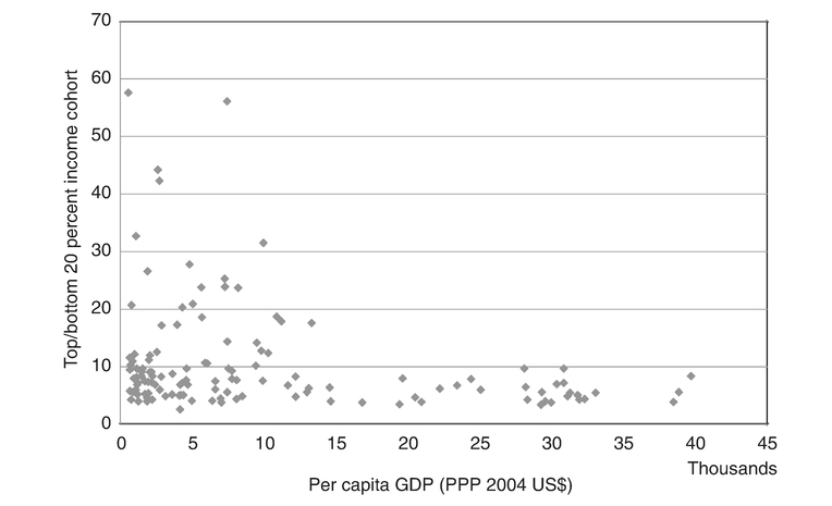
Chart 4.1 Income inequality and per capita GDP.

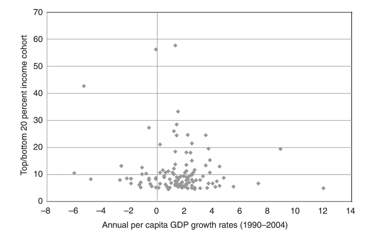
Chart 4.2 Growth and income inequality.

high negative to high positive rates (Chart 4.2). Income inequality does not appear to be necessary for the realization of high levels of per capita income and growth.⁵

The estimates presented here are consistent with the view that high levels of income inequality and increases in income inequality are not necessary conditions for high levels of per capita output and labor productivity. Moreover, these estimates are consistent with the view that less income inequality need not yield low levels of per capita GDP and labor productivity or low growth rates of these variables. These estimates also cast doubt on the view that increasing rates of technical change have been responsible for increasing levels of income in equality.⁶ The behavioral model discussed in this chapter and in Chapters 2 and 3 provides one possible explanation for how more equity, driven by increases in wages, is consistent with high levels of per capita GDP and labor productivity and with higher rates of economic growth.

The conventional wisdom

The conventional wisdom assumes that the economy is x-efficient in terms of effort inputs and also in terms of the choice of technology. What is meant by x-efficiency is that the economy is assumed to be always operating along the production possibility frontier. Effort per unit of input is therefore maximized and cost minimizing technology is adopted in this scenario, thereby maximizing output per person, irrespective of the system of industrial relations in place within the firm and related rates of labor compensation (Leibenstein 1966, 1978, 1979; see also Chapters 1 and 2).⁷ It is therefore assumed that effort discretion does not exist in terms of economic agents having some choice over how hard or how well they work. On the other hand, effort discretion is a necessary condition for the existence of x-inefficiency. It is facilitated by the existence of incomplete contracts (based on their transaction costs) and different behavioral functions especially between employees or the agents of the firm, and members of the firm hierarchy or its principles (Akerlof and Yellen 1986; Altman 1996; Miller 1992; Stiglitz 1987). The conventional wisdom also assumes that the rate of technological change is determined exogenously, outside the causal boundaries of the model. All told, it is assumed that there are no large bills lying around just waiting to be picked up. Society is doing the best it can, given the constraints faced by economic agents, such as imperfect information and transaction costs. The conventional model is therefore consistent with a fundamental principle of contemporary economic theory which McCloskey has referred to as the American Question or the Axiom of Modest Greed:

This is what conventional economic theory predicts rational economic agents must do. If they do not, then market forces will make them do it. The big bill hunters and gatherers will out-compete their relatively lazy competitors and drive them into economic purgatory or to the production possibility frontier (Altman 1999d; Reder 1982). In other words, for firms to remain competitive firms must be x-efficient.

The conventional assumption with regards to x-efficiency in production yields important analytical predictions with regards to the potential economic impact and the welfare implications of income redistribution. These analytical predictions are, in turn, embedded in the concept of Pareto Optimality, which serves as a basis for public policy discussions related to income redistribution. Within this modeling framework, absence the existence of relative price distortions and, therefore, the existence of allocative efficiency and given the assumption of x-efficiency, it follows that income redistribution is a zero-sum game: that which goes to labor, for example, reduces the income to employers. Pareto Optimality, the best of all possible economic worlds, is given by the realization of the joint conditions of allocative and x-efficiency. Given the assumption that income redistribution has no effect on efficiency, any existing income distribution at hand is not considered to be of economic importance since it is assumed that one cannot and should not make interpersonal comparison of the utility attached to a particular distribution. It is assumed without any empirical backing, for example, that the marginal utility of real income is the same for both the poor and the rich. So, income redistribution cannot, by assumption, yield increases in aggregate social utility or welfare.⁸ On the other hand, if it is assumed that income redistribution negatively affects efficiency, income redistribution has the dynamic effect of reducing savings and therefore growth and can, therefore, be critiqued from a positive analytical perspective (Altman 2000a).

In contrast to this conventional perspective on income redistribution, the argument flowing from the behavioral model of economic growth is that there need not be an equity-efficiency trade-off in a competitive market economy to the extent that wages positively affect productivity and do not increase production costs. Therefore, shifting from a low to a high wage economy can be welfare improving. This behavioral model of economic welfare, which is interconnected with the behavioral model of growth, paints a dynamic picture of economic welfare in contradistinction to the static framework provided by Pareto Optimality. In this dynamic scenario, the conditions of Pareto Optimality need not be violated, in the sense that it becomes possible to redistribute income to the relatively less well off without, in the long run, reducing the economic welfare of the relatively well-to-do. Indeed, such redistribution might serve to induce increasing efficiency and technological change thereby increasing the economic welfare of all members of society.

From the perspective of the Edgeworth Box diagram, increasing the real income or nonpecuniary benefits to workers in period t₀ serves to increase the size of the economic pie in period t₁, through its dynamic effect on economic efficiency. In Figure 4.1, if x-efficiency is assumed and C_XIH_XI is the production possibility frontier for cars and housing, any redistribution of income yields a reduction in economic welfare to at least one individual—a clear violation of Pareto Optimality. This would be the case, for example, if income is reallocated from individual a to b yielding a change in the equilibrium distribution of income (zero allocative inefficiencies) from e₀ to e₁. However, if C_XIH_XI is an x-inefficient production possibility frontier, a redistribution of income from a to b might result in an increase in the level of x-efficiency, shifting the frontier for cars and housing outward to C_XEH_XE. In this scenario, income redistribution need not result in there being any losers to the extent that the economic pie is sufficiently expanded. Moreover, income distribution is here consistent in a dynamic sense with the conditions of Pareto Optimality.

An important footnote to this discussion is Pigou’s analysis of market economies which argues for income distribution away from high income individuals to the extent that a dollar shifted in this direction has a higher marginal product for lower income individuals in terms of productivity effects from higher food intake, improved health, and improved or higher levels of human capital. Pigou argues that increasing the income of the less well-to-do serves to improve their productivity, by enhancing their capacities as workers by improving the nutritional levels and health of workers. In addition, investing in the education and skill upgrading of labor also has the effect of increasing labor productivity (Pigou 1952, Ch. 10). But Pigou argues that workers do not have the means to optimally invest in their education. Firms do not have the incentive to optimally

Figure 4.1 Pareto optimality, income distribution and x-efficiency.

invest in general on-the-job training of their workers. Such investment would yield a rate of return, in terms of increased labor productivity that would greatly exceed the return of investing in plant and equipment. Investing in the health and nurture of the sick will also yield high returns by improving the capacity of workers (Pigou 1952, pp. 746–749). He writes:

Education and the general training of workers is connected to investments in the nourishment, housing, and medical care of the children, if education is to build up their productive capacities. A poorly fed, housed, and sickly child could not effectively learn (Pigou 1952, pp. 751–754). In effect, Pigou speaks to market failures with regards to the investment in human capital formation.

Such market failures are now an important topic of analysis in recent efforts to explain why less income inequality is not necessarily connected with a poorer growth record (Aghion 1998; Aghion et al. 1999; Osberg 1995). This Pigouvian type analysis in effect argues that income redistribution increases the size of the economic pie as government intervenes to correct for systematic market failures. Hence, redistributing income need not negatively impact on economic growth or on the level of real per capita income realized in the affected economies. This being said, the focus of this chapter is not on the economic significance of Pig-ouvian type income redistributions in a world of market imperfections. Rather, the focus here is upon changes in income inequality that are independent and unrelated to these types of market imperfections. What is of concern here is how labor market related institutions can affect the distribution of income and how this might be efficiency and, thereby, growth enhancing.

The behavioral alternative

In the behavioral model of the firm discussed in detail in Chapters 2 and 3, unlike in the conventional wisdom, effort discretion exists. Effort inputs are increased as wages and or working conditions improve. Only under an ideal system of industrial relations are effort inputs maximized and, therefore, x-efficiency achieved. In the absence of material gains to the decision makers, for example, in terms of lower unit costs or increased profits, the realization of x-efficiency can be obtained only if the preferences of the decision makers shift toward an x-efficient consistent system of industrial relation.⁹ I also assume that technological change (whether or not a firm adopts an available technology) is a function of, or is induced by, relative production costs (see Chapter 3).¹⁰

In the behavioral model presented in Chapters 2 and 3, unlike in the conventional model, unit costs need not be affected by changes in factor prices, inclusive of the price of labor which serves here as a proxy for all labor related costs. X-inefficient firms can survive even with perfect product markets if wage rates differ between firms and if the differences in wage rates are neutralized by compensating differences in productivity, driven by differences in effort input or technological change. Given technology, at least for an array of wage rates, there may be a unique unit cost of production. On the flip side, there need not be any unique wage rate or labor compensation package that minimizes costs or maximizes the level of profits. Induced technological change only reinforces this argument. Given the assumptions of the model, a low wage regime goes hand in hand with a low productivity regime and a high wage regime goes hand in hand with a high productivity regime and the two wage regimes need not necessarily yield any differences in unit costs or even in rates of return. In this case, high wage firms can compete with low wage firms by becoming more productive, where output is a function of effort per unit of labor input as well as of labor, capital, and “technical change.”

The details of this argument are presented in Chapters 3 and 4 and can be illustrated in Figure 4.2. There is a unique average cost CO₀ that is associated with an array of labor costs or wage and other labor costs up to W₁ where

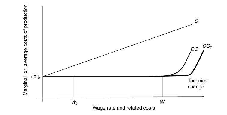
Figure 4.2 Labor and production costs.

diminishing returns set in with respect to the relationship between effort inputs and these labor costs. Up to W₁ effort increases sufficiently to compensate for any increase in labor costs. On the other hand, effort diminishes as one moves from W₁ toward zero, sufficiently to offset any potential gains to the firm that might accrue from lower wages, working conditions, and other related labor costs. At W₁ x-efficiency in production is achieved. Further, increases in labor costs can be compensated for through induced technological change, discussed in Chapter 3. Technological change serves to shift the unit cost curve to the right to CO_T.

In the behavioral model presented here, employers have no material incentive to become more x-efficient if this accrues to them no advantage in terms of unit costs, profits, or own-income. As discussed in Chapter 2, making workers more efficient is a costly process. And, most firms have not adopted the available and known more x-efficient systems of industrial relations because workers often eat up the productivity gains from their increased efficiency. If this were not the case, rational firm decision makers would choose to design a more x-efficient firm, especially if subject to competitive product market forces. There is also a disincentive to become more x-efficient if this involves a loss of power and prestige within the firm to employers as well as the reduction in the percentage of the firm’s labor force that consists of management. In this scenario, an economy would be x-inefficient, even given the availability of relatively x-efficient alternatives, resulting in a loss of income to society at large. X-inefficiency is here a product of the rational private choices made by the firm’s decision makers. The firm can be induced into adopting more efficient methods of firm organization as labor costs rise or as preferences of firm decision makers shift toward more x-efficiency in production.

Income distribution

The behavioral model of the firm and growth presented here has implications for an understanding of the evolution of income distribution through historical time and the distribution of income distributions across economies at a particular point in time.¹¹ Referring back to our discussion of Pareto Optimality, the behavioral model suggests that increasing workers’ wages can positively affect productivity growth and thereby the level of per capita output, this without negatively affecting the income of the other group income claimants within the firm. Wherever this type of modeling scenario applies, first period income redistribution that is a product of increasing the income or in-firm benefits to employees is not only consistent with economic growth, it also contributes to economic growth. It is simply a product of increased x-efficiency and technological progress, discussed above. In this scenario, it is possible to increase the income of one individual or group of individuals without reducing the income of another. Therefore, income redistribution need not be a zero-sum game and it can be consistent with Pareto Optimality seen from a dynamic perspective.

The behavioral model predicts that because a positive causal relationship exists between labor costs and labor productivity as well as total factor productivity, it is highly unlikely that increasing wage inequality is a necessary condition for per capita economic growth. At a minimum, maintaining low real wage growth of the least paid workers is a highly unlikely necessary condition for per capita economic growth. Moreover, under reasonable assumptions, one would expect that such growth is consistent with lower levels of wage inequality. Given, that wage inequality is a key determinant of income inequality one would also expect that when wage inequality diminishes so should income inequality. But this need not always hold true. For example, as already discussed, increasing divorce rates and, related to this, increasing atomization of families, can contribute toward increasing income inequality, holding wage inequality constant. So would an increasing correlation between the income of husbands and wives, holding wage inequality constant (Burtless 1999, 2001). Moreover, income distribution becomes more unequal independent of changes in wage inequality when employment rates and hours worked changes differentially in favor of the higher income groups. Thus, even if there are no changes in wage inequality, income inequality increases when employment rates and hours worked change at either the bottom or the top end of the income distribution (Osberg 2001). This being, said the behavioral model predicts that high levels income inequality or increasing levels of income inequality are not necessary conditions to economic prosperity and growth.

In a simple behavioral model, where x-inefficiency exists and technical change are induced by labor costs, and assuming one homogeneous output and two income groups, workers and employers, wage inequality is reduced within the firm as the wage rate increases. This is illustrated in Table 4.1, in the Sector One dynamics, where wage inequality drops from 5 to 3.4 as wages increase.

If one assumes that minimum wage legislation and unions drive the income of workers, then in this scenario wage inequality is reduced through such interventions in the economy and increased when such interventions are reduced or eliminated. Bear in mind that in the behavioral model introducing or increasing existing minimum wages, and successful union efforts to increase labor compensation and improve working conditions need not increase unit costs or reduce profits. Other variables might also have affected the extent of wage inequality, but the behavioral model suggests the importance of legislative or institutional interventions to this process (Fortin and Lemieux 1997; Freeman 1996; Atkinson 1997). One would also expect that both minimum wages and unions to positively affect the growth process whereas their removal or weakening should contribute to the slowing of economic growth. This type of scenario can also be applied to discuss the possible effects of low unemployment rate policy upon income in equality, a point elaborated upon empirically by Galbraith (1998). In this case, lower unemployment rates affect most significantly the wages of the lowest paid least well-organized workers, thereby increasing their wage relative to those of the higher income workers and other claimants on income. This increase in wages, not only serves to reduce wage inequality, but in the behavioral model it is paid for through the increased productivity that generates. These results easily translate to a multisector model where one sector is high wage and low inequality and the other is low wage and high inequality. In Table 4.1, Panel 6, simply by increasing the wage in Sector Two (the low wage sector), wage inequality is reduced and productivity is enhanced. Reducing the wage in Sector Two, on the other hand, serves to increase inequality and diminish labor productivity. Note that in these scenarios, it is not income redistribution that is driving changes in income distribution. Rather, it is the relative improvements in workers’ income joined with improvements in productivity that yields reduction in income inequality.

In another scenario, with more than one sector, it is clear that the evolution of inequality critically depends upon what occurs within sectors and changes, if any, in the relative importance of the sector within the economy, a point made decades ago by Kuznets (1955) in his classic work on income inequality. Although the behavioral model predicts less wage and income inequality when wages rise, this need not take place in a multi-sector economy where wages are increasing in one sector while diminishing in another. Here, the results are ambiguous, much depending on the extent of wage changes in the sectors and changes in the relative importance of the sectors (Table 4.1, Panels 1 and 2). Even in a scenario where wages are increasing in one sector, with consequent reductions in inequality (say as a result of unionization and tight labor markets), while inequality remains stable in the high inequality sectors, inequality increases if the high inequality sectors become relatively more important (Table 4.1, Panel 3). In this case, mean wages might be increasing in the economy as a whole, while inequality is increasing as well, as a result of a change in the relative importance of the different sectors to the economy. On the other hand, in equality diminishes as a consequence of reducing the relative importance of the high inequality sectors (Table 4.1, Panels 4, 5, and 8). Inequality can also increase as the high wage sector leads the growth process. In this scenario, the wage gap between the high paid workers in the high wage sector and the low wage workers in the low wage sector increases. In this case, to the extent that the low wage workers are x-inefficient, the wage gap could be reduced by introducing minimum wages, for example, which serves to increase the wages for the lowest paid workers thereby keeping wage inequality from increasing to the extent that it would otherwise increase.

The behavioral model is also consistent with a scenario that typifies economies where important outputs are exported and the price of these exports can be subject to price shocks. In such an economy real wages might be increasing and wage inequality decreasing in the domestic sector. However, in the export sector, if positive price shocks result in the income of the employers increasing, this can cause an economy-wide increase in wage inequality (Table 4.1, Panel 7). In this case, increasing mean wage inequality is consistent with both increasing wages in at least one sector and increasing measured income in the economy. Of course such increasing inequality need not occur if employees are able to capture some of the rents achieved in the export sector as a result of positive price shocks.

At a more specific level, the behavioral model also speaks to the potential role of human capital formation in terms of formal education and skill formation, age structure, and technical change as possible determinants of income inequality. If one assumes that all economic agents are homogeneous and producing an identical product using an identical technology, in a world of x-efficiency, all economic agents should be paid the same wage (representing all forms of labor compensation) in long-run competitive product market equilibrium. In other words, in this scenario, the marginal product would be identical for all workers with wages equalized across all workers. But this scenario simply establishes an “ideal type.” In a world where x-inefficiency prevails differentially across firms as a product of different institutional parameters faced by firms and of different work cultures or systems of industrial relations adopted by firms, wages need not be identical in long run equilibrium. Higher wage firms are relatively more x-efficient and, therefore, cost competitive, with the relatively low wage and x-inefficient firms. So, for example, wages can be higher for unionized workers in what would be the relatively more x-efficient firms than in the relatively x-inefficient non-unionized shops. In other words, otherwise identical workers would be receiving different wage rates.¹² This would have the effect of causing a certain level of wage inequality that is unnecessary from the perspective of technical constraints (production function) faced by the firm.

But even if human capital factors, age distribution, and technology, dictate a particular inequality in the distribution of income in an x-efficient long-run equilibrium, the distribution of income predicted in such an x-efficient scenario need not be obtained in a world where x-inefficiency exists. The key point here is that even if the technical constraints within the firm dictate a Gini coefficient of 0.3, a Gini of 0.5 (a Gini of 0 represents perfect equality) might be obtained if different firms are characterized by different work cultures such that one set of firms pay higher wages and is more x-efficient than another. The relatively low wage firms are simply paying workers less than need be given the existence of organizationally induced x-inefficiency. Technical factors such as human capital and technology only set the parameters within which wage or income distribution levels must fall. But according to the behavioral model, whether the minimum inequality allowed for by these technical parameters is realized depends on how the firm is organized. And this, in turn, is affected by institutional parameters such as unions, minimum wages, social goods like unemployment insurance, and employment policy.

More specifically, for example, human capital formation need not generate increasing real income to those with more human capital vested in them, from the perspective of the behavioral model. Nor need the convergence in levels of human capital yield a convergence in wage rates (Herzenberg et al. 1998). On the other hand, a divergence in levels of human capital need not yield a divergence in wage rates. In point of fact, convergence in formal education has not resulted in the convergence of incomes (O’Neill 1995; Parente and Prescott 2000). For one, higher levels of human capital yield higher wages and higher level of productivity, depending on the production function in which it is contained. PhDs employed in fast food restaurants, for example, will not earn high wages. In the behavioral model, human capital endowments, vested in the overall production function of the firm, sets the outerbound parameters to the productivity a worker can achieve, ceteris paribus. Some workers can produce below potential and earn below potential, no matter their human capital endowment, depending upon the organizational parameters of the firm. Such x-inefficiency can yield more income inequality than need be. For example, workers with a high school education or less, might earn less than is necessary, given their potential productivity, in the absence of minimum wage legislation (Fortin and Lemieux 1997; Freeman 1996). In a behavioral model, ceteris paribus, introducing or increasing minimum wages, within limits, can serve to increase the level of x-efficiency and induce technical change, allowing for the higher wages to be cost competitive whilst also serving to reduce income inequality.

Conclusion

The behavioral model of the firm suggests that labor market conditions and how the firm is organized play an important causal role in determining productivity, per capita output differentials, and in determining the extent of income inequality. Where labor costs and firm organization affect the efficiency of the firm, high wage firms can be cost competitive with low wage firms, union firms with nonunion firms, and, more generally, high wage economies can be cost competitive with low wage economies. Moreover, in this behavioral analytical framework, increasing income equality need not be a zero-sum game when output increases as a consequence of increasing labor income. The size of the economic pie increases as the level of x-efficiency increases. In this case, a more equal distribution of income is consistent with and a contributing factor to higher rates of growth and higher levels of per capita output. In this scenario, more wage or income equality need not be at someone else’s expense since more income equality is not achieved through the process of income redistribution, at least in a multi-period framework. Related to this, institutional factors, such as minimum wages, unions, and tight labor market policy can serve not only to reduce wage income inequality, but also toward making an economy relatively more efficient. Finally, from a behavioral perspective, the extent of wage and income inequality is not simply a product of technical parameters embodied in the traditional production function, it is also affected by institutional variables. The production function only sets the outer boundary within which an array of income distributions, all of which are cost competitive, can be realized. This type of modeling of the firm and economy suggests a greater degree of freedom in the determination of the extent of income inequality, from the perspective of public policy and economic analysis, than is suggested by more traditional perspectives where income redistribution and, more generally, more income equality, is at best a zero- sum game and, at worst, a cause of economic inefficiency.

There are some direct public policy implications of the behavioral model for issues related to income distribution. First and foremost, the behavioral model suggests that to the extent that there is an efficiency or technological change effect that flows from improvements in the material well-being of workers, policy should be designed to encourage such improvements and, moreover, to facilitate the realization of such an efficiency and technological change enhancing effect. For example, minimum wages and unions can serve both to improve the well- being of workers and to improve the productivity performance of the firm. Additionally, from a more macroeconomic perspective, policy that serves to maintain low unemployment rates, by improving the bargaining power of labor, can have an efficiency and technology enhancing effect through the impact that resulting improvements in wages and working conditions might have on the firm’s level of x-efficiency and on its technology. A similar case can be made with regards to maintaining reasonable unemployment insurance as well as social insurance programs, both of which affect the bargaining power of labor. However, the behavioral model does not infer that efficiency and technology enhancing effects automatically or costlessly flow from improvements in material level of well-being of workers. Government policy which facilitates firms adopting and investing in improvements in industrial relations, the skill enhancement of workers, and the development and adoption of new technology or the adoption of existing relatively more productive technologies, facilitate firms realizing higher levels of productivity to, at a minimum, offset the higher costs accruing from improvements in labor compensation.

None of these policies are redistributive in nature. Rather, they are geared toward building a more productive economy in a manner where workers, inclusive of those at the lower deciles of the income distribution, capture a significant share of an increasing economic pie. As a consequence of the dynamic relationship, specified by the behavioral model, between labor compensation and economic efficiency and growth, facilitated by government policy, the distribution of income can become more equal over time. But it is not more income equality, per se, that generates more efficiency and growth. In the behavioral model discussed here, causality runs from efficiency and growth to more income equality, where increased income equality is a likely outcome of a more productive economy built upon improvements in the material well-being of workers.