
PART III: PROBLEMS
Section 4.1
4.1.1 Consider Example 4.1. It was suggested to apply the test statistic ![]() (X) = I{X ≤ 18}. What is the power of the test if (i) θ = .6; (ii) θ = .5; (iii) θ = .4? [Hint: Compute the power exactly by applying the proper binomial distributions.]
(X) = I{X ≤ 18}. What is the power of the test if (i) θ = .6; (ii) θ = .5; (iii) θ = .4? [Hint: Compute the power exactly by applying the proper binomial distributions.]
4.1.2 Consider the testing problem of Example 4.1 but assume that the number of trials is n = 100.
4.1.3 Suppose that X has a Poisson distribution with mean λ. Consider the hypotheses H0: λ = 20 against H1: λ ≠ 20.
Section 4.2
4.2.1 Let X1, …, Xn be i. i. d. random variables having a common negative–binomial distribution NB(![]() , ν), where ν is known.
, ν), where ν is known.
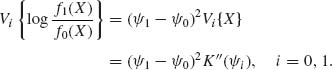
4.2.2 Let X1, X2, …, Xn be i. i. d. random variables having a common distribution Fθ belonging to a regular family. Consider the two simple hypotheses H0: θ = θ0 against H1: θ = θ1; θ0 ≠ θ1. Let ![]() = varθi {log (f(X1; θ1)/f(X1;θ0))}, i = 0, 1, and assume that 0 <
= varθi {log (f(X1; θ1)/f(X1;θ0))}, i = 0, 1, and assume that 0 < ![]() < ∞, i = 0, 1. Apply the Central Limit Theorem to approximate the MP test and its power in terms of the Kullback–Leibler information functions I(θ0, θ1) and I(θ1, θ0), when the sample size n is sufficiently large.
< ∞, i = 0, 1. Apply the Central Limit Theorem to approximate the MP test and its power in terms of the Kullback–Leibler information functions I(θ0, θ1) and I(θ1, θ0), when the sample size n is sufficiently large.
4.2.3 Consider the one–parameter exponential type family with p. d. f. f(x; ![]() ) = h(x) exp {
) = h(x) exp {![]() x1 − K(
x1 − K(![]() )}, where K(
)}, where K(![]() ) is strictly convex having second derivatives at all
) is strictly convex having second derivatives at all ![]()
![]() Ω, i. e., K″(
Ω, i. e., K″(![]() ) > 0 for all
) > 0 for all ![]()
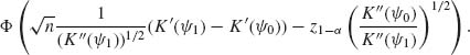
![]() Ω, where Ω is an open interval on the real line. For applying the asymptotic results of the previous problem to test H0:
Ω, where Ω is an open interval on the real line. For applying the asymptotic results of the previous problem to test H0: ![]() ≤
≤ ![]() 0 against H1:
0 against H1: ![]() ≥
≥ ![]() 1, where
1, where ![]() 0 <
0 < ![]() 1, show
1, show
4.2.4 Let X1, X2, …, Xn be i. i. d. random variables having a common negative–binomial distribution NB(p, ν), ν fixed. Apply the results of the previous problem to derive a large sample test of size α of H0: p ≤ p0 against H1: p ≥ p1, 0 < p0 < p1 < 1.
4.2.5 Let X1, X2, …, Xn be i. i. d. random variables having a common distribution with p. d. f. f(x;μ, θ) = (1 − θ)![]() (x) + θ
(x) + θ ![]() (x − μ), −∞ < x < ∞, where μ is known, μ > 0; 0 ≤ θ ≤ 1; and
(x − μ), −∞ < x < ∞, where μ is known, μ > 0; 0 ≤ θ ≤ 1; and ![]() (x) is the standard normal p. d. f.
(x) is the standard normal p. d. f.
4.2.6 Let X1, …, Xn be i. i. d. random variables having a common continuous distribution with p. d. f. f(x;θ). Consider the problem of testing the two simple hypotheses H0: θ = θ0 against H1: θ = θ1, θ0 ≠ θ1. The MP test is of the form ![]() (x) = I{Sn ≥ c}, where Sn =
(x) = I{Sn ≥ c}, where Sn = ![]() log (f(Xi; θ1)/f(Xi; θ0)). The two types of error associated with
log (f(Xi; θ1)/f(Xi; θ0)). The two types of error associated with ![]() c are
c are
![]()
A test ![]() c* is called minimax if it minimizes max (
c* is called minimax if it minimizes max (![]() 0(c),
0(c), ![]() 1(c)). Show that
1(c)). Show that ![]() c is minimax if there exists a c* such that
c is minimax if there exists a c* such that ![]() 0(c* ) =
0(c* ) = ![]() 1(c*).
1(c*).
Section 4.3
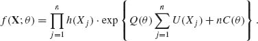
4.3.1 Consider the one–parameter exponential type family with p. d. f. s
![]()
where Q′(θ) > 0 for all θ ![]() Θ; Q(θ) and C(θ) have second order derivatives at all θ
Θ; Q(θ) and C(θ) have second order derivatives at all θ ![]() Θ.
Θ.
4.3.2 Let X1, …, Xn be i. i. d. random variables having a scale and location parameter exponential distribution with p. d. f.
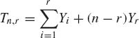
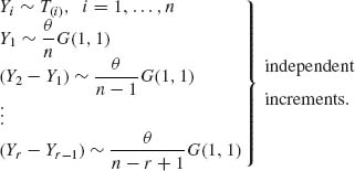
4.3.3 Consider n identical systems that operate independently. It is assumed that the time till failure of a system has a  distribution. Let Y1, Y2, …, Yr be the failure times until the rth failure.
 is distributed like
 4.3.4 Consider the linear regression model prescribed in Problem 3, Section 2.9. Assume that α and σ are known.
Section 4.4
4.4.1 Let X1, …, Xn be i. i. d. random variables having an N(0, σ2) distribution. Determine the UMP unbiased test of size α of H0: σ2 = ![]() against H1: σ2 ≠
against H1: σ2 ≠ ![]() , where 0 <
, where 0 < ![]() < ∞.
< ∞.
4.4.2 Let X ~ B(20, θ), 0 < θ < 1. Construct the UMP unbiased test of size α = .05 of H0: θ = .15 against H1: θ ≠ .15. What is the power of the test when θ = .05, .15, .20, .25
4.4.3 Let X1, …, Xn be i. i. d. having a common exponential distribution G(![]() , 1), 0 < θ < ∞. Consider the reliability function ρ = exp { − t/θ }, where t is known. Construct the UMP unbiased test of size α for H0: ρ = ρ0 against H1: ρ ≠ ρ0, for some 0 < ρ0 < 1.
, 1), 0 < θ < ∞. Consider the reliability function ρ = exp { − t/θ }, where t is known. Construct the UMP unbiased test of size α for H0: ρ = ρ0 against H1: ρ ≠ ρ0, for some 0 < ρ0 < 1.
Section 4.5
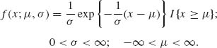
4.5.1 Let X1, …, Xn be i. i. d. random variables where X1 ~ ξ + G(![]() , 1), −∞ < ξ < ∞, 0 < σ < ∞. Construct the UMPU tests of size α and their power function for the hypotheses:
, 1), −∞ < ξ < ∞, 0 < σ < ∞. Construct the UMPU tests of size α and their power function for the hypotheses:
4.5.2 Let X1, …, Xm be i. i. d. random variables distributed like N(μ1, σ2) and let Y1, …, Yn be i. i. d. random variables distributed like N(μ2, σ2); −∞ < μ1, μ2 < ∞; 0 < σ 2 < ∞. Furthermore, the X–sample is independent of the Y–sample. Construct the UMPU test of size α for
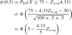
4.5.3 Let X1, …, Xn be i. i. d. random variables having N(μ, σ2) distribution. Construct a test of size α for H0: μ + 2σ ≥ 0 against μ + 2σ < 0. What is the power function of the test?
4.5.4 In continuation of Problem 3, construct a test of size α for
![]()
4.5.5 Let (X1, X2) have a trinomial distribution with parameters (n, θ1, θ2), where 0 < θ1, θ2 < 1, and θ1 + θ2 ≤ 1. Construct the UMPU test of size α of the hypotheses H0: θ1 = θ2; H1: θ1 ≠ θ2.
4.5.6 Let X1, X2, X3 be independent Poisson random variables with means λ1, λ2, λ3, respectively, 0 < λi < ∞ (i = 1, 2, 3). Construct the UMPU test of size α of H0: λ1 = λ2 = λ3; H1: λ1 > λ2 > λ3.
Section 4.6
4.6.1 Consider the normal regression model of Problem 3, Section 2.9. Develop the likelihood ratio test, of size ![]() , of
, of
4.6.2 Let (![]() 1, S
1, S![]() ), …, (
), …, (![]() k,
k, ![]() ) be the sample mean and variance of k independent random samples of size n1, …, nk, respectively, from normal distributions N(μi,
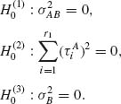
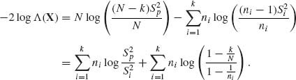
) be the sample mean and variance of k independent random samples of size n1, …, nk, respectively, from normal distributions N(μi, ![]() ), i = 1, …, k. Develop the likelihood ratio test for testing H0: σ1 = ··· = σk; μ1, …, μk arbitrary against the general alternative H1: σ1, …, σk and μ1, …, μk arbitrary. [The test that rejects H0 when
), i = 1, …, k. Develop the likelihood ratio test for testing H0: σ1 = ··· = σk; μ1, …, μk arbitrary against the general alternative H1: σ1, …, σk and μ1, …, μk arbitrary. [The test that rejects H0 when 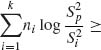
![]() [k−1], where
[k−1], where ![]() =
= 
![]() and N =
and N = ![]() ni, is known as the Bartlett test for the equality of variances (Hald, 1952, p. 290).]
ni, is known as the Bartlett test for the equality of variances (Hald, 1952, p. 290).]
4.6.3 Let (X1, …, Xk) have a multinomial distribution MN(n, θ), where θ = (θ1, …, θk), 0 < θi < 1, ![]() θi = 1. Develop the likelihood ratio test of H0: θ1 = ··· = θk =
θi = 1. Develop the likelihood ratio test of H0: θ1 = ··· = θk = ![]() against H1: θ arbitrary. Provide a large sample approximation for the critical value.
against H1: θ arbitrary. Provide a large sample approximation for the critical value.
4.6.4 Let (Xi, Yi), i = 1, …, n, be i. i. d. random vectors having a bivariate normal distribution with zero means and covariance matrix ![]() , = σ2
, = σ2 ![]() , 0 < σ2 < ∞, −1 < ρ < 1. Develop the likelihood ratio test of H0: ρ = 0, σ arbitrary against H1: ρ ≠ 0, σ arbitrary.
, 0 < σ2 < ∞, −1 < ρ < 1. Develop the likelihood ratio test of H0: ρ = 0, σ arbitrary against H1: ρ ≠ 0, σ arbitrary.
4.6.5 Let (x11, Y11), …, (X1n, Y1n) and (x21, Y21), …, (x2n, Y2n) be two sets of independent normal regression points, i. e., Yij ~ N(α1 + β1xj, σ2), j = 1, …, n and Y2j ~ N(α2 +β2 xj;σ2), where x(1) = (x11, …, x1n)′ and x(2) = (x21, …, x2n)′ are known constants.
4.6.6 The one–way analysis of variance (ANOVA) developed in Section 4.6 corresponds to model (<4.), which is labelled Model I. In this model, the incremental effects are fixed. Consider now the random effects model of Example 3.9, which is labelled Model II. The analysis of variance tests H0: τ2 = 0, σ2 arbitrary; against H1: τ2 > 0, σ2 arbitrary; where τ2 is the variance of the random effects a1, …, ar. Assume that all the samples are of equal size, i. e., n1 = ··· = nr = n.
4.6.7 Consider the two–way layout model of ANOVA (4.6.33) in which the incremental effects of ![]() , are considered fixed, but those of B,
, are considered fixed, but those of B, ![]() , are considered i. i. d. random variables having a N(0,
, are considered i. i. d. random variables having a N(0, ![]() ) distribution. The interaction components
) distribution. The interaction components ![]() are also considered i. i. d. (independent of
are also considered i. i. d. (independent of ![]() ) having a N(0,
) having a N(0, ![]() ) distribution. The model is then called a mixed effect model. Develop the ANOVA tests of the null hypotheses
) distribution. The model is then called a mixed effect model. Develop the ANOVA tests of the null hypotheses
What are the power functions of the various F–tests (see Scheffé, 1959, Chapter 8)?
Section 4.7
4.7.1 Apply the X2–test to test the significance of the association between the attributes A, B in the following contingency table
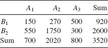
At what level of significance, α, would you reject the hypothesis of no association?
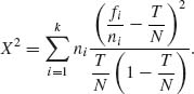
4.7.2 The X2–test statistic (4.7.5) can be applied in large sample to test the equality of the success probabilities of k Bernoulli trials. More specifically, let f1, …, fk be independent random variables having binomial distributions B(ni, θi), i = 1, …, k. The hypothesis to test is H0: θ1 = ··· = θk = θ, θ arbitrary against H1: the θs are not all equal. Notice that if H0 is correct, then 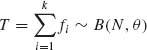 where N =
 ![]() ni. Construct the 2 × k contingency table
ni. Construct the 2 × k contingency table
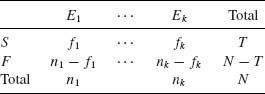
This is an example of a contingency table in which one margin is fixed (n1, …, nk) and the cell frequencies do not follow a multinomial distribution. The hypothesis H0 is equivalent to the hypothesis that there is no association between the trial number and the result (success or failure).
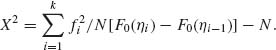
4.7.3 The test statistic X2, as given by (4.7.5) can be applied to test also whether a certain distribution F0(x) fits the frequency distribution of a certain random variable. More specifically, let Y be a random variable having a distribution over (a, b), where a could assume the value −∞ and/or b could assume the value +∞. Let η0 < η1 < ··· < ηk with η0 = a and ηk = b, be a given partition of (a, b). Let fi (i = 1, …, k) be the observed frequency of Y over (ηi−1, ηi) among N i. i. d. observations on Y1, …, Yn, i. e., fi = ![]() I{ηi−1 < Yj ≤ ηi}, i = 1, …, k. We wish to test the hypothesis H0: FY(y) ≡ F0(y), where FY(y) denotes the c. d. f. of Y. We notice that if H0 is true, then the expected frequency of Y at [ηi−1, ηi] is ei = N{F0(ηi) − F0(ηi−1)}. Accordingly, the test statistic X2 assumes the form
I{ηi−1 < Yj ≤ ηi}, i = 1, …, k. We wish to test the hypothesis H0: FY(y) ≡ F0(y), where FY(y) denotes the c. d. f. of Y. We notice that if H0 is true, then the expected frequency of Y at [ηi−1, ηi] is ei = N{F0(ηi) − F0(ηi−1)}. Accordingly, the test statistic X2 assumes the form
The hypothesis H0 is rejected, in large samples, at level of significance α if X2 ≥ ![]() [k−1]. This is a large sample test of goodness of fit, proposed in 1900 by Karl Pearson (see Lancaster, 1969, Chapter VIII; Bickel and Doksum, 1977, Chapter 8, for derivations and proofs concerning the asymptotic distribution of X2 under H0).
[k−1]. This is a large sample test of goodness of fit, proposed in 1900 by Karl Pearson (see Lancaster, 1969, Chapter VIII; Bickel and Doksum, 1977, Chapter 8, for derivations and proofs concerning the asymptotic distribution of X2 under H0).
The following 50 numbers are so–called “random numbers” generated by a desk calculator: 0.9315, 0.2695, 0.3878, 0.9745, 0.9924, 0.7457, 0.8475, 0.6628, 0.8187, 0.8893, 0.8349, 0.7307, 0.0561, 0.2743, 0.0894, 0.8752, 0.6811, 0.2633, 0.2017, 0.9175, 0.9216, 0.6255, 0.4706, 0.6466, 0.1435, 0.3346, 0.8364, 0.3615, 0.1722, 0.2976, 0.7496, 0.2839, 0.4761, 0.9145, 0.2593, 0.6382, 0.2503, 0.3774, 0.2375, 0.8477, 0.8377, 0.5630, 0.2949, 0.6426, 0.9733, 0.4877, 0.4357, 0.6582, 0.6353, 0.2173. Partition the interval (0, 1) to k = 7 equal length subintervals and apply the X2 test statistic to test whether the rectangular distribution R(0, 1) fits the frequency distribution of the above sample. [If any of the seven frequencies is smaller than six, combine two adjacent subintervals until all frequencies are not smaller than six.]
4.7.4 In continuation of the previous problem, if the hypothesis H0 specifies a distribution F(x; θ) that depends on a parameter θ = (θ1, …, θr), i ≤ r, but the value of the parameter is unknown, the large sample test of goodness of fit compares
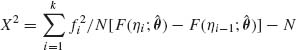
with ![]() [k−1−r] (Lancaster, 1969, p. 148), where
[k−1−r] (Lancaster, 1969, p. 148), where ![]() are estimates of θ obtained by maximizing
are estimates of θ obtained by maximizing
![]()
4.7.5 Consider Problem 3 of Section 2.9. Let (X1i, X2i), i = 1, …, n be a sample of n i. i. d. such vectors. Construct a test of H0: ρ = 0 against H1: ρ ≠ 0, at level of significance α.
Section 4.8
4.8.1 Let X1, X2, … be a sequence of i. i. d. random variables having a common binomial distribution B(1, θ), 0 < θ < 1.
4.8.2 Let X1, X2, … be a sequence of i. i. d. random variables having a N(0, σ2) distribution. Construct the Wald SPRT to test H0: σ2 = 1 against H1: σ2 = 2 with error probabilities α = .01 and β = .07. What is π (σ2) and Eσ2{N} when σ2 = 1.5?
PART IV: SOLUTIONS TO SELECTED PROBLEMS
4.1.2 The sample size is n = 100.
![]()
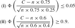
The solution of these 2 equations is n ![]() 82, C
82, C ![]() 55. For these values n and C we have α = 0.066 and
55. For these values n and C we have α = 0.066 and ![]() (0.6) = 0.924.
(0.6) = 0.924.
4.2.1 Assume that ν = 2. The m. s. s. is T = ![]() Xi ~ NB(
Xi ~ NB(![]() , 2n).
, 2n).
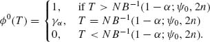
Let T1−α(![]() 0) = NB−1 (1−α ;2n,
0) = NB−1 (1−α ;2n, ![]() 0). Then
0). Then
![]()
![]()
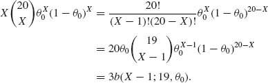
We can compute these functions with the formula
![]()
For ![]() 0 = 0.05, α = 0.10,
0 = 0.05, α = 0.10, ![]() 1 = 0.15, 1−β = 0.8, we get the equations
1 = 0.15, 1−β = 0.8, we get the equations
The solution of these equations is n = 15.303 and t = 3.39. Since n and t are integers we take n = 16 and t = 3. Indeed, P0.05 (T ≤ 3) = I.95(32, 4) = 0.904. Thus,
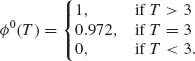
The power at ![]() = 0.15 is
= 0.15 is
![]()
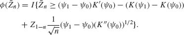
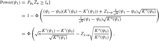
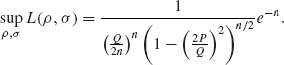
4.2.3
![]()
For ![]() 1 >
1 > ![]() 0,
0,
![]()
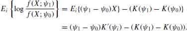
Since Ei{X} = K′(![]() i), i = 0, 1.
i), i = 0, 1.
4.3.1 Since Q′(θ) > 0, if θ1 < θ2 then Q(θ2) > Q(θ1)
![]()
![]()
Thus, the p. d. f. of T(X) is
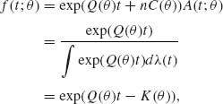
where
![]()
This is a one–parameter exponential type density.
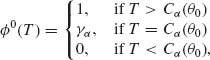
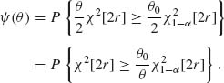
where Cα (θ0) is the (1 − α) quantile of T under θ0. If T is discrete then
![]()
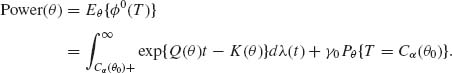
By Karlin’s Lemma, this function is increasing in θ. It is differentiable w. r. t. θ.
4.3.3
Accordingly,
![]()
The left–hand side is equal to ![]() Yi+(n−r)Yr. Thus Tn, r ~
Yi+(n−r)Yr. Thus Tn, r ~ ![]() χ2[2r].
χ2[2r].
![]()
4.4.2 X ~ B(20, θ). H0: θ = .15, H1: θ ≠ .15, α = .05. The UMPU test is
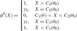
The test should satisfy the conditions
Thus, we find C1, γ1, C2, γ2 from the equations
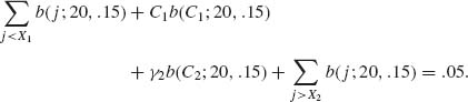
We start with C1 = B−1 (.025;20, .15) = 0, C2 = B−1(.975; 20, .15) = 6
These satisfy (i). We check now (ii).
![]()
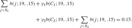
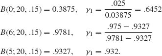
We keep C1, γ1, and C2 and change γ2 to satisfy (ii); we get
![]()
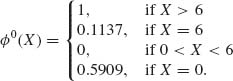
We go back to 1, with γ′2 and recompute γ′1. We obtain γ′1 = .59096. With these values of γ′1 and γ′2, Equation (i) yields 0.049996 and Equation (ii) yields 0.0475. This is close enough. The UMPU test is
4.5.1 X1, …, Xn are i. i. d. ~ μ +σ G(1, 1), −∞ < μ < ∞, 0 < σ < ∞. The m. s. s. is (nX(1), U), where
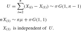
![]()
against
![]()
The m. s. s. for ![]() * is T =
* is T = ![]() Xi = U + nX(1). The conditional distribution of nX(1) given T is found in the following way.
Xi = U + nX(1). The conditional distribution of nX(1) given T is found in the following way.
![]()
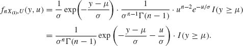
The joint p. d. f. of nX(1)> and U is
We make the transformation
![]()
The joint density of (nX(1), T) is
![]()
Thus, the conditional density of nX(1), given T, is
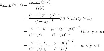
The c. d. f. of nX(1)| T, at μ = μ0 is
![]()
The (1 − α)–quantile of H0(y| t) is the solution y of ![]() = 1 − α, which is Cα (μ0, t) = μ0 +(t − μ0)(1−(1 − α)1/(n−1)). The UMPU test of size α is
= 1 − α, which is Cα (μ0, t) = μ0 +(t − μ0)(1−(1 − α)1/(n−1)). The UMPU test of size α is
![]()
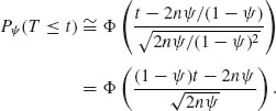
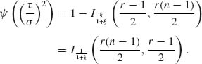
The power function of this test is
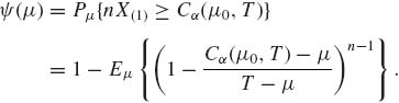
T − μ ~ σ G(1, n). Hence, for ξ = 1 − (1 − α)1/(n−1),
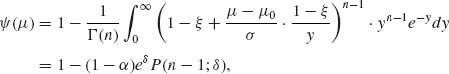
where δ = (μ − μ0)/σ). This is a continuous increasing function of μ.
![]()
The m. s. s. for ![]() * is X(1). Since U is independent of X(1), the conditional test is based on U only. That is,
* is X(1). Since U is independent of X(1), the conditional test is based on U only. That is,
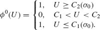
We can start with ![]() [2n−2].
[2n−2].
4.5.4
![]()
against
![]()
Obviously, if μ ≥ 0 then H0 is true. A test of ![]() : μ ≥ 0 versus
: μ ≥ 0 versus ![]() : μ < 0 is
: μ < 0 is
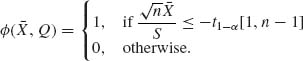
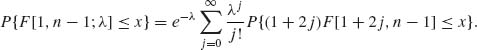
where S2 = Q/(n−1) is the sample variance. We should have a more stringent test. Consider the statistic ![]() ~ F[1, n−1;λ] where λ =
~ F[1, n−1;λ] where λ = ![]() . Notice that for
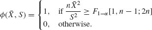
. Notice that for ![]() *, μ2 = 4σ2 or λ0 = 2n. Let θ = (μ, σ). If θ
*, μ2 = 4σ2 or λ0 = 2n. Let θ = (μ, σ). If θ ![]() Θ1, then λ > 2n and if θ
Θ1, then λ > 2n and if θ ![]() Θ0, λ ≤ 2n. Thus, the suggested test is
Θ0, λ ≤ 2n. Thus, the suggested test is
![]()
The distribution of a noncentral F[1, n−1;λ] is like that of (1+2J)F[1+2J, n−1], where J ~ Pois (λ) (see Section 2.8). Thus, the power function is
![]()
The conditional probability is an increasing function of J. Thus, by Karlin’s Lemma, Ψ (λ) is an increasing function of λ. Notice that
Thus, F1-α [1, n−1;λ] ![]() λ.
λ.
4.6.2 The GLR statistic is
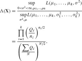
where ![]() .
.
Notice that if n1 = ··· = nk = n, then ![]() n log
n log ![]() = 0. Thus, for large samples, as n→ ∞, the Bartlett test is: reject H0 if
= 0. Thus, for large samples, as n→ ∞, the Bartlett test is: reject H0 if ![]() ni
ni ![]() ≥
≥ ![]() [k − 1]. We have k−1 degrees of freedom since σ2 is unknown.
[k − 1]. We have k−1 degrees of freedom since σ2 is unknown.
4.6.4
![]()
Let Q = ![]() (
(![]() +
+ ![]() ) and P =
) and P = ![]() XiYi. H0: ρ = 0, σ2 arbitrary; H1: ρ ≠ 0, σ2 arbitrary. The MLE of σ2 under H0 is
XiYi. H0: ρ = 0, σ2 arbitrary; H1: ρ ≠ 0, σ2 arbitrary. The MLE of σ2 under H0 is ![]() . The likelihood of (ρ, σ2) is
. The likelihood of (ρ, σ2) is
![]()
Thus, ![]() L(0, σ2) =
L(0, σ2) = ![]() exp (−n). We find now
exp (−n). We find now ![]() 2 and
2 and ![]() that maximize L(ρ, σ2). Let l(ρ, σ2) = log L(ρ, σ2)
that maximize L(ρ, σ2). Let l(ρ, σ2) = log L(ρ, σ2)
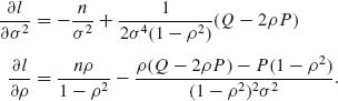
Equating these partial derivatives to zero, we get the two equations

Solution of these equations gives the roots ![]() 2 =
2 = ![]() and
and ![]() =
= ![]() . Thus,
. Thus,
It follows that
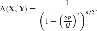
Λ (X, Y) is small if ![]() is small or P is close to zero.
is small or P is close to zero.
4.6.6 Model II of ANOVA is
![]()
where ![]() independent of {ai}.
independent of {ai}.
Notice that Xij| ai ~ N(μ +ai, σ2). Hence, Xij ~ N(μ, σ2 + τ2). Moreover,
![]()
and
![]()
![]()
Thus,
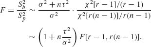
![]()
Let
![]()
Thus,
where ![]() and
and ![]() are independent.
are independent.
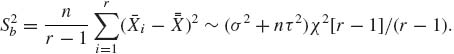
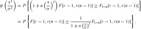
![]()
Hence,
![]()
Let ![]() . Thus,
. Thus,
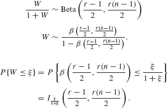
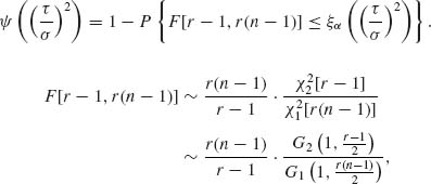
Let ![]() . Then
. Then
1. We also call such a test a boundary α–similar test.