Chapter 6: Model to Production and Beyond

In the last chapter, we discussed model training and prediction for online and batch models with Feast. For the exercise, we used the Feast infrastructure that was deployed to the AWS cloud during the exercises in Chapter 4, Adding Feature Stores to ML Models. During these exercises, we looked at how Feast decouples feature engineering from model training and model prediction. We also learned how to use offline and online stores during batch and online prediction.

In this chapter, we will reuse the feature engineering pipeline and the model built in Chapter 4, Adding Feature Stores to ML Models, and Chapter 5, Model Training and Inference, to productionize the machine learning (ML) pipeline. The goal of this chapter is to reuse everything that we have built in the previous chapters, such as Feast infrastructure on AWS, feature engineering, model training, and model-scoring notebooks, to productionize the ML model. As we go through the exercises, it will give us an opportunity to look at how early adoption of Feast not only decoupled the ML pipeline stages but also accelerated the production readiness of the ML model. Once we productionize the batch and online ML pipelines, we will look at how the adoption of Feast opens up opportunities for other aspects of the ML life cycle, such as feature monitoring, automated model retraining, and also how it can accelerate the development of a future ML model. This chapter will help you understand how to productionize the batch and online models that use Feast, and how to use Feast for feature drift monitoring and model retraining.

We will discuss the following topics in order:

• Setting up Airflow for orchestration
• Productionizing a batch model pipeline
• Productionizing an online model pipeline
• Beyond model production

Technical requirements

To follow the code examples in the chapter, the resources created in Chapter 4, Adding Feature Store to ML Models, and Chapter 5, Model Training and Inference, are required. You will need familiarity with Docker and any notebook environment, which could be a local setup, such as Jupyter, or an online notebook environment, such as Google Colab, Kaggle, or SageMaker. You will also need an AWS account with full access to some of the resources, such as Redshift, S3, Glue, DynamoDB, and the IAM console. You can create a new account and use all the services for free during the trial period. You can find the code examples of the book and feature repository in the following GitHub links:

• https://github.com/PacktPublishing/Feature-Store-for-Machine-Learning/tree/main/Chapter06
• https://github.com/PacktPublishing/Feature-Store-for-Machine-Learning/tree/main/customer_segmentation

Setting up Airflow for orchestration

To productionize the online and batch model, we need a workflow orchestration tool that can run the ML pipelines for us on schedule. There are a bunch of tools available, such as Apache Airflow, AWS Step Functions, and SageMaker Pipelines. You can also run it as GitHub workflows if you prefer. Depending on the tools you are familiar with or offered at your organization, orchestration may differ. For this exercise, we will use Amazon Managed Workflows for Apache Airflow (MWAA). As the name suggests, it is an Apache Airflow-managed service by AWS. Let's create an Amazon MWAA environment in AWS.

Important Note

Amazon MWAA doesn't have a free trial. You can view the pricing for the usage at this URL: https://aws.amazon.com/managed-workflows-for-apache-airflow/pricing/. Alternatively, you can choose to run Airflow locally or on EC2 instances (EC2 has free tier resources). You can find the setup instructions to run Airflow locally or on EC2 here:

Airflow local setup: https://towardsdatascience.com/getting-started-with-airflow-locally-and-remotely-d068df7fcb4

Airflow on EC2: https://christo-lagali.medium.com/getting-airflow-up-and-running-on-an-ec2-instance-ae4f3a69441

S3 bucket for Airflow metadata

Before we create an environment, we need an S3 bucket to store the Airflow dependencies, Directed Acyclic Graphs (DAGs), and so on. To create an S3 bucket first, please follow the instructions in the Amazon S3 for storing data subsection of Chapter 4, Adding Feature Store to ML Models. Alternatively, you can also choose to use an existing bucket. We will be creating a new bucket with the name airflow-for-ml-mar-2022. In the S3 bucket, create a folder named dags. We will be using this folder to store all the Airflow DAGs.

The Amazon MWAA provides multiple different ways to configure additional plugins and Python dependencies to be installed in the Airflow environment. Since we need to install a few Python dependencies to run our project, we need to tell Airflow to install these required dependencies. One way of doing it is by using the requirements.txt file. The following code block shows the contents of the file:

papermill==2.3.4

boto3==1.21.41

ipython==8.2.0

ipykernel==6.13.0

apache-airflow-providers-papermill==2.2.3

Save the contents of the preceding code block in a requirements.txt file. We will be using papermill (https://papermill.readthedocs.io/en/latest/) to run the Python notebooks. You can also extract code and run the Python script using the bash or python operator available in Airflow.

Important Note

If you are running Airflow locally, make sure that the library versions are compatible with the Airflow version. The Amazon MWAA Airflow version at the time of writing is 2.2.2.

Once you have the requirement.txt file created, upload it into the S3 bucket we have created. We will be using it in the next section during the environment creation.

Amazon MWAA environment for orchestration

Now that we have the required resources for creating the Amazon MWAA environment, let's follow the following steps to create the environment:

1. To create a new environment, log in to your AWS account and navigate to the Amazon MWAA console using the search bar in the AWS console. Alternatively, visit https://us-east-1.console.aws.amazon.com/mwaa/home?region=us-east-1#environments. The following web page will be displayed:

Figure 6.1 – The Amazon MWAA environments console

2. On the page displayed in Figure 6.1, click on the Create environment button, and the following page will be displayed:

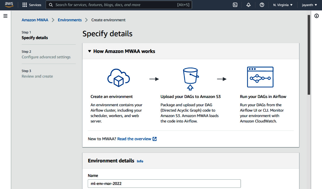
Figure 6.2 – Amazon MWAA environment details

3. Provide a name for the Amazon MWAA environment on the page displayed in Figure 6.2. Scroll down to the DAG code in Amazon S3 section; you should see the following parameters on the screen:

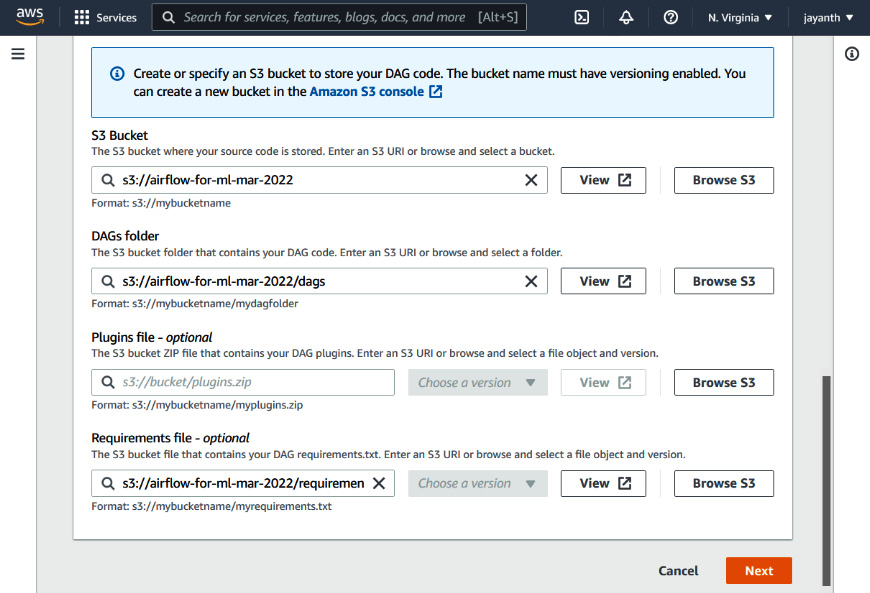
Figure 6.3 – Amazon MWAA – the DAG code in S3 section

4. On the screen displayed in Figure 6.3, enter the S3 bucket in the textbox or use the Browse S3 button. Here, we will use the S3 bucket that we created earlier in the section. Once you select the S3 bucket, the other fields will appear. For DAGs folder, select the folder that we created earlier in the S3 bucket. Also, for the Requirements file - optional field, browse for the requirements.txt file that we uploaded or enter the path to the file. As we don't need any plugins to run the project, we can leave the optional Plugins file field blank. Click on the Next button:

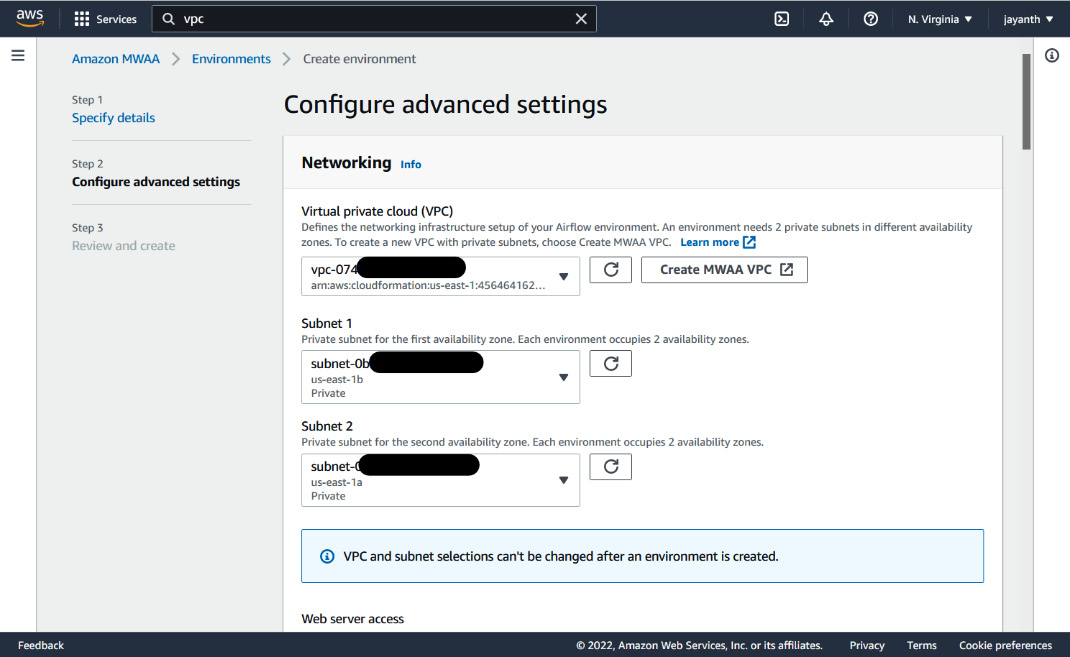
Figure 6.4 – Amazon MWAA advanced settings

5. The next page displayed is shown in Figure 6.4. For Virtual private cloud (VPC), select the available default VPC from the dropdown. One caveat here is that the selected VPC should have at least two private subnets. If it doesn't have the private subnets, when you try to select Subnet 1 and Subnet 2, you will notice that all the options are grayed out. If you run into this scenario, click on Create MWAA VPC. It will take you to the CloudFormation console; once you have filled in the form with all the parameters, follow through and click on Create stack. It will create a VPC that can be used by Amazon MWAA. Once the VPC is created, come back to this window and select the new VPC and subnets, and continue.
6. After selecting the VPC, for Web server access, select Public network; leave everything else to default, and scroll all the way down. In the Permissions section, you will notice that it says it will create a new role for Amazon MWAA. Make a note of the role name. We will have to add permissions to this role later. After that, click on Next.
7. On the next page, review all the input provided, scroll all the way down, and click on Create environment. It will take a few minutes to create the environment.
8. Once the environment is created, you should be able to see the environment in the Available state on the Amazon MWAA environments page. Pick the environment that we just created and click on the Open Airflow UI link. An Airflow home page will be displayed, similar to the one in the following figure:
   

Figure 6.5 – The Airflow UI

9. To test whether everything is working fine, let's quickly create a simple DAG and look at how it works. The following code block creates a simple DAG with a dummy operator and a Python operator:

   from datetime import datetime

   from airflow import DAG

   from airflow.operators.dummy_operator import DummyOperator

   from airflow.operators.python_operator import PythonOperator

   def print_hello():

       return 'Hello world from first Airflow DAG!'

   dag = DAG('hello_world',

             description='Hello World DAG',

             schedule_interval='@daily',

             start_date=datetime(2017, 3, 20),

             catchup=False)

   start = DummyOperator(task_id="start", dag=dag)

   hello_operator = PythonOperator(

       task_id='hello_task',

       python_callable=print_hello,

       dag=dag)

   start >> hello_operator

10. The DAG defined in the preceding code is pretty simple; it has two tasks – start and hello_operator. The start task is a DummyOperator, does nothing, and is used for making the DAG look pretty on the UI. The hello_operator task just invokes a function that returns a message. In the last line, we define a dependency between the operators.
11. Copy the preceding code block, save the file as example_dag.py, and upload it to the dags folder in S3 that we created earlier. (My S3 location is s3://airflow-for-ml-mar-2022/dags.) Once you upload it, it should appear in the Airflow UI within seconds. The following figure displays the Airflow UI with the DAG:

Figure 6.6 – The Airflow UI with the example DAG

12. By default, the DAGs are disabled; hence, when you visit the page, you may not see the exact page such as the one displayed in Figure 6.6. Enable the DAG by clicking on the toggle button in the left-most column. Once enabled, DAG will run for the first time and update the run results. You can also trigger the DAG using the icon in the Links column. Click on the hello_world hyperlink in the DAG column in the UI. You will see the details page of the DAG with different tabs. Feel free to play around and look at the different options available on the details page.  
13. The following figure displays the graph view of the DAG:

Figure 6.7 – The graph view of the DAG

14. Now that we have verified that Airflow is set up correctly, let's add the required permissions for Airflow to run the ML pipeline.
15. If you recall, during the last step of environment creation (the paragraph following Figure 6.4), we made note of the role name the Airflow environment is using to run the DAGs. Now, we need to add permissions to the role. To do so, navigate to the AWS IAM roles console page using the search function or visit https://us-east-1.console.aws.amazon.com/iamv2/home?region=us-east-1#/roles. In the console, you should see the IAM role that is associated with the Airflow environment. Select the IAM role; you should see the following page:

Figure 6.8 – The Amazon MWAA IAM role

Important Note

If you didn't make a note, you can find the role name in the environment details page on the AWS console.

16. In Figure 6.8, click on Add permissions; from the dropdown, select Attach policies, and you will be taken to the following page:

Figure 6.9 – IAM – Attach policies

17. On the web page, search and select the following policies – AmazonS3FullAccess, AWSGlueConsoleFullAccess, AmazonRedshiftFullAccess, and AmazonDynamoDBFullAccess. Once the policies are selected, scroll down and click on Attach policies to save the role with the new policies.

    Important Note

    It is never a good idea to assign full access to any of the resources without restrictions. When you run an enterprise application, it is recommended to restrict access based on the resources, such as read-only access to a specific S3 bucket and DynamoDB tables.

    If you are running Airflow locally, you can use the IAM user credential in the notebook.

Now that our orchestration system is ready, let's look at how to use it to productionize the ML pipeline.

Productionizing the batch model pipeline

In Chapter 4, Adding Feature Store to ML Models, for model training, we used the features ingested by the feature engineering notebook. We also created a model-scoring notebook that fetches features for a set of customers from Feast and runs predictions for it using the trained model. For the sake of the experiment, let's assume that the raw data freshness latency is a day. That means the features need to be regenerated once a day, and the model needs to score customers against those features once a day and store the results in an S3 bucket for consumption. To achieve this, thanks to our early organization and decoupling of stages, all we need to do is run the feature engineering and model scoring notebook/Python script once a day consecutively. Now that we also have a tool to perform this, let's go ahead and schedule this workflow in the Airflow environment.

The following figure displays how we will be operationalizing the batch model:

Figure 6.10 – Operationalization of the batch model

As you can see in the figure, to operationalize the workflow, we will use Airflow to orchestrate the feature-engineering and model-scoring notebooks. The raw data source for feature engineering, in our case, is the S3 bucket where online-retail.csv is stored. As we have already designed our scoring notebook to load the production model from the model repo (in our case, an S3 bucket) and store the prediction results in a S3 bucket, we will reuse the same notebook. One thing you might notice here is that we are not using the model-training notebook for every run; the reason is obvious – we want to run predictions against a version of the model that has been validated, tested, and also met our performance criteria on the test data.

Before scheduling this workflow, I have done minor changes to the feature-engineering notebook and model-prediction notebooks. The final notebooks can be found at the following GitHub URL: https://github.com/PacktPublishing/Feature-Store-for-Machine-Learning/blob/main/Chapter06/notebooks/(ch6_feature_engineering.ipynb,ch6_model_prediction.ipynb). To schedule the workflow, download the final notebooks from GitHub and upload them to an S3 bucket that we created earlier, as an Airflow environment will need to access these notebooks during runs. I will upload it to the following location: s3://airflow-for-ml-mar-2022/notebooks/.

Important Note

AWS secret access key and an S3 path – I have commented out AWS credentials in both the notebooks, as we are adding permissions to an Amazon MWAA IAM role. If you are running it in local Airflow, please uncomment and add secrets. Also, update the S3 URLs wherever necessary, as the S3 URLs point to the private buckets that I have created during the exercises.  

Feature repo – As we have seen before, we must clone the feature repo so that the Feast library can read the metadata. You can follow the same git clone (provided that git is installed) approach or set up a GitHub workflow to push the repo to S3 and download the same in the notebook. I have left both code blocks in the notebook with comments. You can use whichever is convenient.

S3 approach – To use an S3 download approach, clone the repo in your local system and run the following commands in the Linux terminal to upload it to a specific S3 location:

export AWS_ACCESS_KEY_ID=<aws_key>

export AWS_SECRET_ACCESS_KEY=<aws_secret>

AWS_DEFAULT_REGION=us-east-1

aws s3 cp customer_segmentation s3://<s3_bucket>/customer_segmentation --recursive

On successful upload, you should be able to see the folder contents in the S3 bucket.

Now that the notebooks are ready, let's write the Airflow DAG for the batch model pipeline. The DAG will have the following tasks in order – start (dummy operator), feature_engineering (Papermill operator), model_prediction (Papermill operator), and end (dummy operator).

The following code block contains the first part of the Airflow DAG:

from datetime import datetime

from airflow import DAG

from airflow.operators.dummy_operator import DummyOperator

from airflow.providers.papermill.operators.papermill import PapermillOperator

import uuid

dag = DAG('customer_segmentation_batch_model', 

          description='Batch model pipeline', 

          schedule_interval='@daily', 

          start_date=datetime(2017, 3, 20), catchup=False)

In the preceding code block, we have defined the imports and DAG parameters such as name, schedule_interval, and start_date. The schedule_interval='@daily' schedule says that the DAG should run daily.

The following code block defines the rest of the DAG (the second part), which contains all the tasks and the dependencies among them:

start = DummyOperator(task_id="start", dag=dag)

run_id = str(uuid.uuid1())

feature_eng = PapermillOperator(

    task_id="feature_engineering",

    input_nb="s3://airflow-for-ml-mar-2022/notebooks/ch6_feature_engineering.ipynb",

    output_nb=f"s3://airflow-for-ml-mar-2022/notebooks/runs/ch6_feature_engineering_{ run_id }.ipynb",

    dag=dag,

    trigger_rule="all_success"

)

model_prediction = PapermillOperator(

    task_id="model_prediction",

    input_nb="s3://airflow-for-ml-mar-2022/notebooks/ch6_model_prediction.ipynb",

    output_nb=f"s3://airflow-for-ml-mar-2022/notebooks/runs/ch6_model_prediction_{run_id}.ipynb",

    dag=dag,

    trigger_rule="all_success"

)

end = DummyOperator(task_id="end", dag=dag, 

                    trigger_rule="all_success")

start >> feature_eng >> model_prediction >> end

As you can see in the code block, there are four steps that will execute one after the other. The feature_engineering and model_prediction steps are run using PapermillOperator. This takes the path to the S3 notebook as input. I have also set an output path to another S3 location so that we can check the output notebook of each run. The last line defines the dependency between the tasks. Save the preceding two code blocks (the first and second parts) as a Python file and call it batch-model-pipeline-dag.py. After saving the file, navigate to the S3 console to upload the file into the dags folder that we pointed our Airflow environment to in Figure 6.3. The uploaded file is processed by the Airflow scheduler. When you navigate to the Airflow UI, you should see the new DAG called customer_segmentation_batch_model on the screen.

The following figure displays the Airflow UI with the DAG:

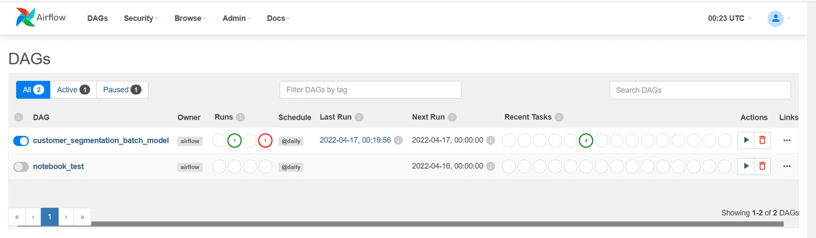
Figure 6.11 – The batch model DAG on Airflow

As we have not enabled the DAG by default option during the Airflow environment creation (which can be set in Airflow configuration variables in Amazon MWAA), when the DAG appears on the UI for the first time, it will be disabled. Click on the toggle button on the left-most column to enable it. Once enabled, the DAG will run for the first time. Click on the customer_segmentation_batch_model hyperlink to navigate to the details page, and feel free to look around to see the different visualization and properties of the DAG. If you navigate to the Graph tab, the DAG will be displayed, as shown in the following screenshot:

Figure 6.12 – The batch model DAG graph view

In Figure 6.12, you can see the graph view of the DAG. If there were any failures in the last run, they will appear in red outline. You can also view the logs of successful execution or failures for each of the tasks. As all the tasks are green, this means everything went well. You can also see the results of the last few runs in Figure 6.11. Airflow also provides you with the history of all the runs.

Now that the task run is complete, we can go and check the output notebook, the S3 bucket for the new set of features, or the S3 bucket for the new set of predictions. All three should be available after successful runs. Here, we will be verifying just the prediction results folder, but feel free to verify the others as well.

Important Note

In case of any failures, verify the logs for the failed tasks (click on the failed task in graph view to see available information). Check the permissions for Amazon MWAA, the S3 paths for input/output, and also whether all the requirements are installed in the Amazon MWAA environment.

The following screenshot shows the new prediction results in an S3 bucket:

Figure 6.13 – The prediction results in an S3 bucket

In addition, you can also do all kinds of fancy things with Airflow, such as sending email notifications for failure, Slack notifications for daily runs, and integration with PagerDuty. Feel free to explore the options. Here is a list of supported providers in Airflow: https://airflow.apache.org/docs/apache-airflow-providers/packages-ref.html.

Now that our batch model is running in production, let's look at how to productionize the online model with Feast.

Productionizing an online model pipeline

In the previous chapter, for the online model, we built REST endpoints to serve on-demand predictions for customer segmentation. Though the online model is hosted as a REST endpoint, it needs a supporting infrastructure for the following functions:

• To serve features in real time (we have Feast for that)
• To keep features up to date (we will use the feature-engineering notebook with Airflow orchestration for this)

In this chapter, we will continue from where we left off and use the feature-engineering notebook built in Chapter 4, Adding Feature Store to ML Models, in combination with a notebook to synchronize offline data to an online store in Feast.

The following figure shows the operationalization of the online model pipeline:

Figure 6.14 – The operationalization of the online model

As you can see in Figure 6.14, we will use Airflow for the orchestration of feature engineering; data freshness is still one day here, and scheduling can be done for a shorter duration. Feast can also support streaming data if there is a need. The following URL has an example you can use: https://docs.Feast.dev/reference/data-sources/push. The REST endpoints developed in Chapter 5, Model Training and Inference, will be Dockerized and deployed as a SageMaker endpoint.

Important Note

Once Dockerized, the Docker image can be used to deploy into any containerized environment, such as Elastic Container Service, Elastic BeanStalk, and Kubernetes. We are using SageMaker, as it takes less time to set up and also has advantages such as data capture and IAM authentication that come out of the box.

Orchestration of a feature engineering job

As we already have two notebooks (feature engineering and sync offline to online store) and we are familiar with Airflow, let's schedule the feature engineering workflow first. Again, in the notebook, I have done some minor changes. Please verify the changes before using it. You can find the notebooks (ch6_feature_engineering.ipynb and ch6_sync_offline_online.ipynb) here: https://github.com/PacktPublishing/Feature-Store-for-Machine-Learning/tree/main/Chapter06/notebooks. Just the way we did it for the batch model, download the notebooks and upload them to a specific S3 location. I will be uploading them to the same location as before: s3://airflow-for-ml-mar-2022/notebooks/. Now that the notebooks are ready, let's write the Airflow DAG for the online model pipeline. The DAG will have the following steps in order – start (dummy operator), feature_engineering (Papermill operator), sync_offline_to_online (Papermill operator), and end (dummy operator).

The following code block contains the first part of the Airflow DAG:

from datetime import datetime

from airflow import DAG

from airflow.operators.dummy_operator import DummyOperator

from airflow.providers.papermill.operators.papermill import PapermillOperator

dag = DAG('customer_segmentation_online_model', 

          description='Online model pipeline', 

          schedule_interval='@daily', 

          start_date=datetime(2017, 3, 20), catchup=False)

Just like in the case of the batch model pipeline DAG, this contains the DAG parameters.

The following code block defines the rest of the DAG (the second part), which contains all the tasks and the dependencies among them:

start = DummyOperator(task_id="start")

run_time = datetime.now()

feature_eng = PapermillOperator(

    task_id="feature_engineering",

    input_nb="s3://airflow-for-ml-mar-2022/notebooks/ch6_feature_engineering.ipynb",

    output_nb=f"s3://airflow-for-ml-mar-2022/notebooks/runs/ch6_feature_engineering_{run_time}.ipynb",

    trigger_rule="all_success",

    dag=dag

)

sync_offline_to_online = PapermillOperator(

    task_id="sync_offline_to_online",

    input_nb="s3://airflow-for-ml-mar-2022/notebooks/ch6_sync_offline_online.ipynb",

    output_nb=f"s3://airflow-for-ml-mar-2022/notebooks/runs/ch6_sync_offline_online_{run_time}.ipynb",

    trigger_rule="all_success",

    dag=dag

)

end = DummyOperator(task_id="end", trigger_rule="all_success")

start >> feature_eng >> sync_offline_to_online >> end

The structure of the Airflow DAG is similar to the batch model DAG we looked at earlier; the only difference is the third task, sync_offline_to_online. This notebook syncs the latest features from offline data to online data. Save the preceding two code blocks (the first and second parts) as a Python file and call it online-model-pipeline-dag.py. After saving the file, navigate to the S3 console to upload the file into the dags folder that we pointed our Airflow environment to in Figure 6.3. As with the batch model, the uploaded file is processed by the Airflow scheduler, and when you navigate to the Airflow UI, you should see the new DAG called customer_segmentation_online_model on the screen.

The following screenshot displays the Airflow UI with the DAG:

Figure 6.15 – The Airflow UI with both the online and batch models

To enable the DAG, click on the toggle button on the left-most column. Once enabled, the DAG will run for the first time. Click on the customer_segmentation_online_model hyperlink to navigate to the details page, and feel free to look around to see the different visualization and properties of the DAG. If you navigate to the Graph tab, the DAG will be displayed, as shown in the following screenshot:

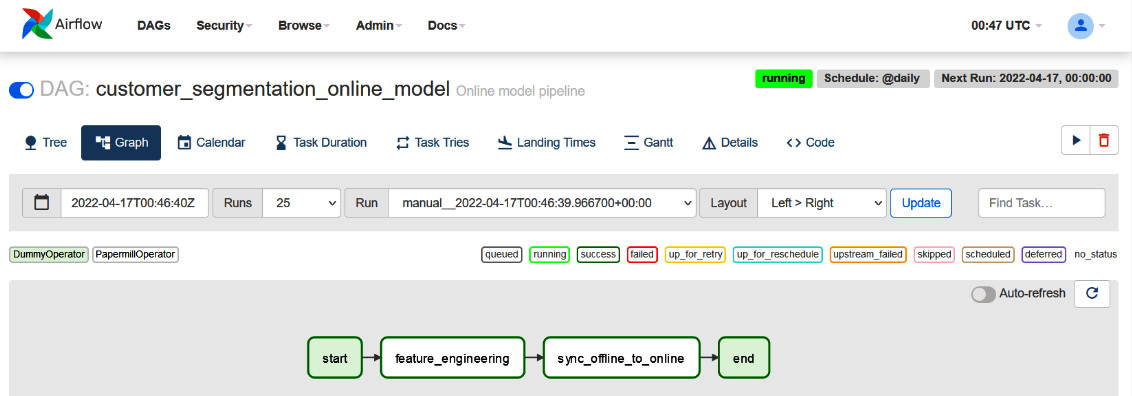
Figure 6.16 – The online model pipeline graph view

As you can see in Figure 6.16, on successful runs, the graph will be green. As discussed during the batch model pipeline execution, you can verify the output notebook, DynamoDB tables, or S3 bucket to make sure that everything is working fine and can also check logs in case of failures.

Now that the first part of the online model pipeline is ready, let's Dockerize the REST endpoints we developed in the previous chapter and deploy them as a SageMaker endpoint.

Deploying the model as a SageMaker endpoint

To deploy the model to SageMaker, we need to first dockerize the REST API we built in Chapter 5, Model Training and Inference. Before we do that, let's create an Elastic Container Registry (ECR), where we can save the Docker image of the model and use it in SageMaker endpoint configurations.

An ECR for the Docker image

To create the ECR resource, navigate to the ECR console from the search bar or use the following URL: https://us-east-1.console.aws.amazon.com/ecr/repositories?region=us-east-1. The following page will be displayed:

Figure 6.17 – The ECR home page

On the page displayed in Figure 6.17, you can choose either the Private or Public repository tab. Then, click on the Create repository button:

Figure 6.18 – ECR – Create repository

I have selected Private here; depending on whether you choose Private or Public, the options will change, but either way, it's straightforward. Fill in the required fields, scroll all the way down, and click on Create repository. Once the repository is created, go into the repository details page, and you should see a page similar to the one shown in Figure 6.19.

Important Note

Private repositories are secured with IAM, whereas public repositories can be accessed by anybody on the internet. Public repositories are mainly used for sharing/open sourcing your work with others outside an organization:

Figure 6.19 – ECR repository details

On the preceding page, click on View push commands, and you should see a popup, similar to the one shown in Figure 6.20:

Figure 6.20 – ECR push commands

Depending on the operating system you are using for building the Docker image, save the necessary commands. We will use these commands to build the Docker image.

Building the Docker image

As mentioned earlier, we will be using the REST endpoints built in the previous chapter in this section. If you recall correctly, we had added two REST endpoints, ping and invocations. These endpoints are not random, though the same can be hosted in any container environment. To host a Docker image in the SageMaker endpoints, the requirement is that it should have the ping (which is the GET method) and invocations (which is the POST method) routes. I have added a couple of files to the same folder structure, which will be useful for building the Docker image. The REST code and folder structure are available at the following URL: https://github.com/PacktPublishing/Feature-Store-for-Machine-Learning/tree/main/online-model-rest-api.

Important Note

The additional files are Dockerfile, requirements.txt, and serve.

Consecutively, clone the REST code to the local system, copy the feature repository into the root directory of the project, export the credentials, and then run the commands in Figure 6.20.

Important Note

You can use the same user credential that was created in Chapter 4, Adding Feature Store to ML Models. However, we had missed adding ECR permissions to the user. Please navigate to the IAM console and add AmazonEC2ContainerRegistryFullAccess to the user. Otherwise, you will get an access error.

The following are the example commands:

cd online-model-rest-api/

export AWS_ACCESS_KEY_ID=<AWS_KEY>

export AWS_SECRET_ACCESS_KEY=<AWS_SECRET>

export AWS_DEFAULT_REGION=us-east-1

aws ecr get-login-password --region us-east-1 | docker login --username AWS --password-stdin <account_number>.dkr.ecr.us-east-1.amazonaws.com

docker build -t customer-segmentation .

docker tag customer-segmentation:latest <account_number>.dkr.ecr.us-east-1.amazonaws.com/customer-segmentation:latest

docker push <account_number>.dkr.ecr.us-east-1.amazonaws.com/customer-segmentation:latest

The commands logs in to ECR using the credentials set in the environment, builds the Docker image, and tags and pushes the Docker image to the registry. Once the image is pushed, if you navigate back to the screen in Figure 6.19, you should see the new image, as shown in the following screenshot:

Figure 6.21 – ECR with the pushed image

Now that the image is ready, copy the image Uniform Resource Identifier (URI) by clicking on the icon next to Copy URI, as shown in Figure 6.21. Let's deploy the Docker image as a SageMaker endpoint next.

Creating a SageMaker endpoint

Amazon SageMaker aims at providing managed infrastructure for ML. In this section, we will only be using the SageMaker inference components. SageMaker endpoints are used for deploying a model as REST endpoints for real-time prediction. It supports Docker image models and also supports a few flavors out of the box. We will be using the Docker image that we pushed into the ECR in the previous section. SageMaker endpoints are built using three building blocks – models, endpoint configs, and endpoints. Let's use these building blocks and create an endpoint next.

A SageMaker model

The model is used to define the model parameters such as the name, the location of the model, and the IAM role. To define a model, navigate to the SageMaker console using the search bar and look for Models in the Inference section. Alternatively, visit https://us-east-1.console.aws.amazon.com/sagemaker/home?region=us-east-1#/models. The following screen will be displayed:

Figure 6.22 – The SageMaker Models console

On the displayed page, click on Create model to navigate to the next screen. The following page will be displayed:

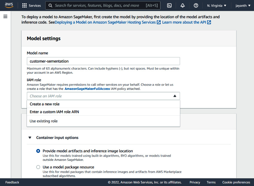
Figure 6.23 – SageMaker – Create model

As shown in Figure 6.23, input a model name, and for the IAM role, select Create a new role from the dropdown. A new popup appears, as displayed in the following screenshot:

Figure 6.24 – The SageMaker model – Create an IAM role

In the popup, leave everything as default for the purpose of this exercise and click on Create role. AWS will create an IAM role, and on the same screen, you should see a message in the dialog with a link to the IAM role. The following figure shows the displayed message:

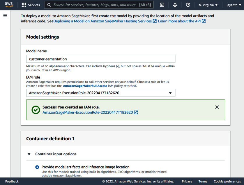
Figure 6.25 – The SageMaker model – the new execution role is created

Now, if you recall correctly, we are using DynamoDB as the online store; as we are reading data on demand from DynamoDB tables, the IAM role needs access to them. Therefore, navigate to the IAM role we just created using the link displayed on the page in a new tab, add AmazonDynamoDBFullAccess, and come back to this tab. Scroll down to the Container definition 1 section, where you should see the following parameters:

Figure 6.26 – The SageMaker model – the Container definition 1 section

For the Location of inference code image parameter, paste the image URI that we copied from the screen, as displayed in Figure 6.21. Leave the others as their defaults and scroll again to the Network section:

Figure 6.27 – The Sagemaker Model – the Network section

Here, select the VPC to Default vpc, select one or two subnets from the list, and choose the default security group. Scroll down to the bottom and click on Create model.

Important Note

It is never a good idea to select the default security group for production deployment, as inbound rules are not restrictive.

Now that the model is ready, let's create the endpoint configuration next.

Endpoint configuration

To set up the endpoint configuration, navigate to the SageMaker console using the search bar and look for Endpoint Configurations in the Inference section. Alternatively, visit https://us-east-1.console.aws.amazon.com/sagemaker/home?region=us-east-1#/endpointConfig. The following page will be displayed:

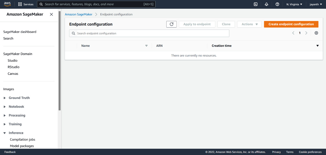
Figure 6.28 – The Sagemaker Endpoint configuration console

On the displayed web page, click on Create endpoint configuration. You will be navigated to the following page:

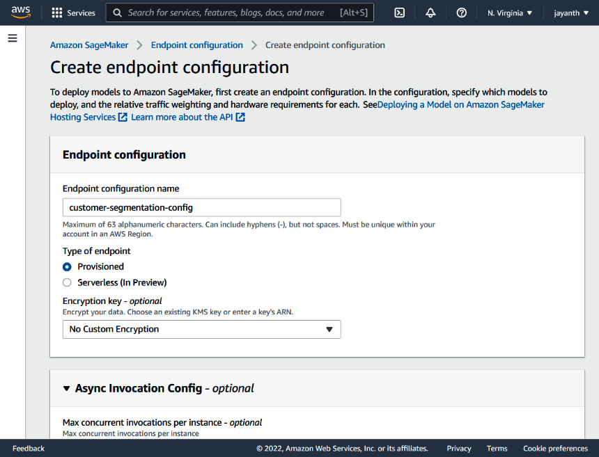
Figure 6.29 – SageMaker – Create endpoint configuration

On this screen, fill in the Endpoint configuration name field; I have given the name customer-segmentation-config. Scroll down to the Data capture section. This is used to define what percent of real-time inference data needs to be captured, where (the S3 location), and how it needs to be stored (JSON or CSV). You can choose to enable this or leave it disabled. I have left it disabled for this exercise. If you enable it, it will ask you for additional information. The section following Data capture is Production variants. This is used for setting up multiple model variants, and A/B testing of the models. For now, since we only have one variant, let's add that here. To add a variant, click on the Add model link in the section; the following popup will appear:

Figure 6.30 – SageMaker – adding a model to the endpoint config

In the popup, select the model that we created earlier, scroll all the way down, and click on Create endpoint configuration.

SageMaker endpoint creation

The last step is to use the endpoint configuration to create an endpoint. To create a SageMaker endpoint, navigate to the SageMaker console using the search bar and look for Endpoints in the Inference section. Alternatively, visit https://us-east-1.console.aws.amazon.com/sagemaker/home?region=us-east-1#/endpoints. The following page will be displayed:

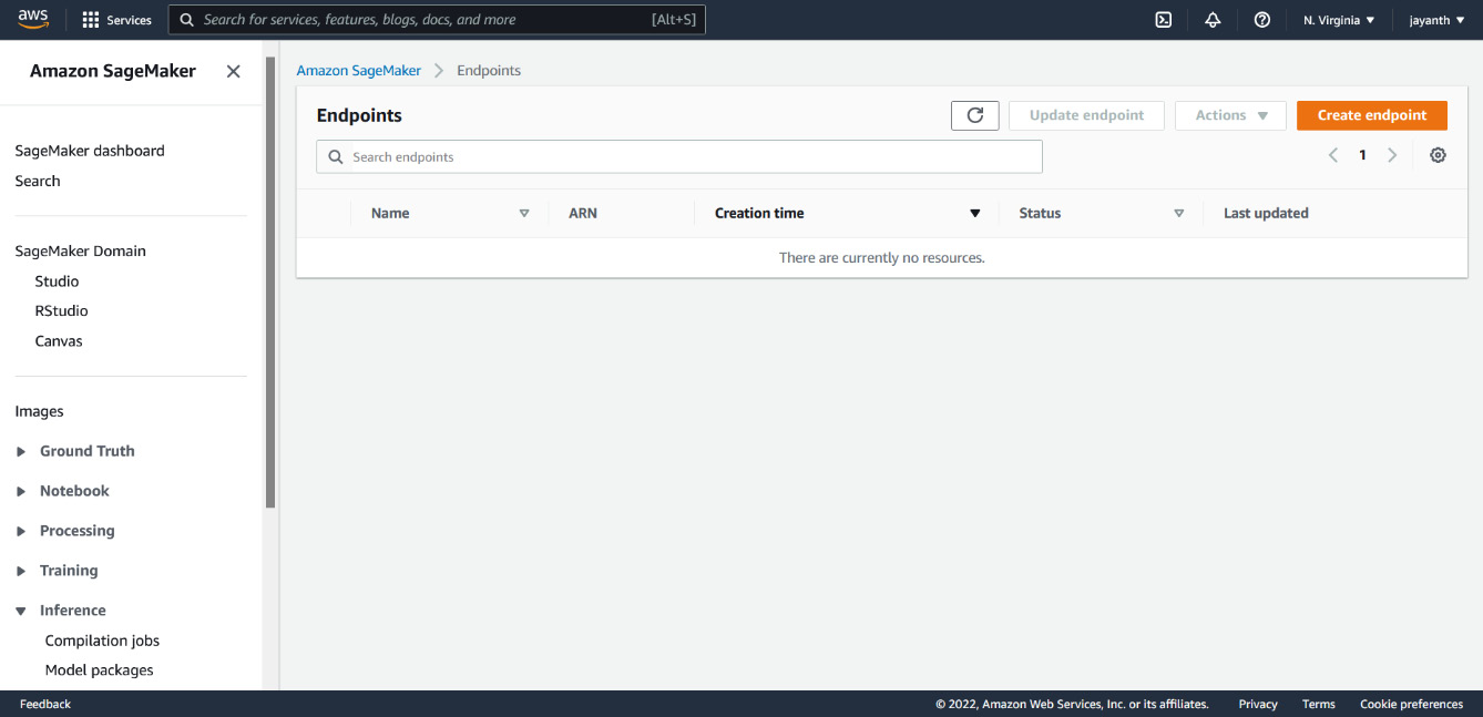
Figure 6.31 – The SageMaker Endpoints console

On the page shown in Figure 6.31, click on Create endpoint to navigate to the following page:

Figure 6.31 – SageMaker – creating an endpoint

On the web page displayed in Figure 6.31, provide an endpoint name. I have given the name customer-segmentation-endpoint. Scroll down to the Endpoint configuration section, select the endpoint configuration we created earlier, and click on the Select endpoint configuration button. Once it is selected, click on Create endpoint. It will take a few minutes to create an endpoint. When the endpoint status changes to Available, your model is live for serving real-time traffic.

Testing the SageMaker endpoint

The next thing we need to know is how to consume the model. There are different ways – you can use the SageMaker library, Amazon SDK client (Python, TypeScript, or any other available), or a SageMaker endpoint URL. All these methods default to AWS IAM authentication. If you have special requirements and want to expose the model without authentication or with custom authentication, it can be achieved using the API gateway and Lambda authorizer. For the purpose of this exercise, we will be using the boto3 client to invoke the API. Irrespective of how we invoke the endpoint, the results should be the same.

The following code block invokes the endpoint using the boto3 client:  

import json

import boto3

import os

os.environ["AWS_ACCESS_KEY_ID"] = "<aws_key>"

os.environ["AWS_SECRET_ACCESS_KEY"] = "<aws_secret>"

os.environ["AWS_DEFAULT_REGION"] = "us-east-1"

payload = json.dumps({"customer_list":["12747.0", "12841.0"]})

runtime = boto3.client("runtime.sagemaker")

response = runtime.invoke_endpoint(

    EndpointName= "customer-segmentation-endpoint", 

    ContentType="application/json", Body=payload

)

response = response["Body"].read()

result = json.loads(response.decode("utf-8"))

print(results)

In the preceding code block, we are invoking the endpoint that we created to run predictions for two customers with the 12747.0 and 12841.0 IDs. The endpoint will respond within milliseconds with the predictions for the given customer IDs. Now, the endpoint can be shared with the model consumers.

Now that the model is in production, let's look at a few aspects that come after a model moves to production.

Beyond model production

In this section, we will discuss the postproduction aspects of ML and how we benefit from the adoption of a feature store.

Feature drift monitoring and model retraining

Once the model is in production, the next question that will come up frequently is how the model is performing in production. There may be different metrics used to measure the performance of a model – for instance, for a recommendation model, performance may be measured by a conversion rate, which is how often the recommended product was purchased. Similarly, predicting the next action of a customer may be measured by error rate, and so on. There is no universal way of doing it. But if a model's performance is bad, it needs to be retrained or replaced with a new one.

One other aspect that defines when a model should be retrained is when the feature starts to drift away from the values with which it was trained. For example, let's say the mean frequency value of the customer during the initial model training was 10, but now, the mean frequency value is 25. Similarly, the lowest monetary value was initially $100.00 and now it is $500.00. This is called data drift.

Data drift monitoring measures the change in the statistical distribution of the data; in the case of feature monitoring, it is comparing the change in the statistical distribution of a feature from t1 time to t2 time. The article at the following URL discusses different metrics for data drift monitoring: https://towardsdatascience.com/automating-data-drift-thresholding-in-machine-learning-systems-524e6259f59f.

With a feature store, it is easy to retrieve a training dataset from two different points in time, namely the dataset used for model training and the latest feature values for all the features used in model training. Now, all we need to do is run data drift monitoring on schedule to generate a drift report. The standardization that Feast brought to the table is, since the data is stored and retrieved using standard APIs, a generic feature drift monitoring can be run on schedule for all the datasets in the feature store. The feature drift report can be used as one of the indicators for model retraining. If feature drift is affecting the model's performance, it can be retrained with the latest dataset, and deployed and AB-tested with the current production model.

Model reproducibility and prediction issues

If you recall from Chapter 1, An Overview of the Machine Learning Life Cycle, model reproducibility is one of the common problems of ML. We need a way to consistently reproduce the model (or training data used for model). Without a feature store, if the underlying raw data that is used to generate features changes, it is not possible to reproduce the same training dataset. However, with a feature store, as we discussed earlier, the features are versioned with a timestamp (one of the columns in the features DataFrame is an event timestamp). Hence, we can query the historical data to generate the same feature set used for model training. If the algorithm used for training the model is not stochastic, the model can also be reproduced. Let's try this out.

Since we have already done something similar to this in the Model training with a feature store section of Chapter 5, Model Training and Inference, we will reuse the same code to run this experiment. Copy and run all the code till you create the entity DataFrame and then replace the event_timestamp column with an older timestamp (the timestamp of when the model was trained), as shown here. In this case, the model was trained at 2022-03-26 16:24:21, as shown in Figure 5.1 of Chapter 5, Model Training and Inference:

## replace timestamp to older time stamp.

entity_df["event_timestamp"] = pd.to_datetime("2022-03-26 16:24:21")

Once you are done replacing the timestamp, continue running the code from the Dee's model training experiments section of Chapter 5, Model Training and Inference. You should be able to generate the exact same dataset that was used in Dee's model training (in this case, the dataset in Figure 5.2 of Chapter 5, Model Training and Inference). Hence, if the model uses a nonrandom algorithm, then the model can also be reproduced using the feature set.

One other advantage of a feature store is the debugging prediction issue. Let's consider a scenario where you have a website-facing model that is classifying a transaction as fraudulent or not. During the peak hour, it flagged a few transactions as fraudulent, but the transactions were legitimate. The customer called in and complained to the customer service department, and now it's the data scientist Subbu's turn to figure out what went wrong. If there was no feature store in the project, to reproduce the issue, Subbu would have to go into the raw data, try to generate the features, and see whether the behavior still remains the same. If not, Subbu would have to go into the application log, process it, look for user behavior before the event, try to reproduce it from the user interaction perspective, and also capture the features for all these trials, hoping that the issue can be reproduced at least once.

On the other hand, with the feature store used in the project, Subbu will figure out the approximate time when the event happened, what the entities and features used in the model are, and what the version of the model that was running in production was at the time of the event. With this information, Subbu will connect to the feature store and fetch all the features used in the model for all the entities for the approximate time range when the issue happened. Let's say that the event occurred between 12:00pm to 12:15pm today, features were streaming, and the freshness interval was around 30 seconds. This means that, on average, for a given entity, there is a chance that features will change in the next 30 seconds from any given time.

To reproduce the issue, Subbu will form an entity DataFrame with the same entity ID repeated 30 times in one column and, for the event time column, a timestamp from 12:00pm to 12:15pm with 30-second intervals. With this entity DataFrame, Subbu will query the historical store using the Feast API and run the prediction for the generated features. If the issue is reproduced, Subbu has the feature set that caused the issue. If not, using the entity DataFrame, the interval will be reduced to less than 30 seconds, maybe to 10 seconds, to figure out if features changed at a faster pace than 30 seconds. Subbu can continue doing this till she finds the feature set that reproduces the issue.

A headstart for the next model

Now that the model has productionized, the data scientist Subbu picks up the next problem statement. Let's assume that the next ML model has to predict the Next Purchase Day (NPD) of a customer. The use case here could be that based on the NPD, we want to run a campaign for a customer. If a customers' purchase day is farther in the future, we want to offer a special deal so that we can encourage purchasing sooner. Now, before going to a raw dataset, Subbu can look for available features based on how the search and discoverability aspect is integrated into the feature store. Since Feast moved from service-oriented to SDK/CLI-oriented, there is a need for catalog tools, a GitHub repository of all the feature repositories, a data mesh portal, and so on. However, in the case of feature stores such as SageMaker or Databricks, users can connect to feature store endpoints (with SageMaker runtime using a boto3 or Databricks workspace) and browse through the available feature definitions using the API or from the UI. I have not used the Tecton feature store before, but Tecton also offers a UI for its feature store that can be used to browse through the available features. As you can see, this is one of the drawbacks of the different versions of Feast between 0.9.X and 0.20.X (0.20 is the version at the time of writing).

Let's assume, for now, that Subbu has a way to locate all the feature repositories. Now, she can connect and browse through them to figure out what the projects and feature definitions are that could be useful in the NPD model. So far, we have just one feature repository that has the customer RFM features that we have been using so far, and these features can be useful in the model. To use these features, all Subbu has to do is get read access to the AWS resource, and the latest RFM features will be available every day for experimentation and can also be used if the model moves to production.

To see how beneficial the feature store would be during the development of the subsequent model, we should try building the NPD. I will go through the initial few steps to get you started on the model. As we followed a blog during the development of the first model, we will be following another part in the same blog series, which can be found at https://towardsdatascience.com/predicting-next-purchase-day-15fae5548027. Please read through the blog, as it discusses the approach and why the author thinks specific features will be useful. Here, we will be skipping ahead to the feature engineering section.

We will be using the feature set that the blog author uses, which includes the following:

• RFM features and clusters
• The number of days between the last three purchases
• The mean and standard deviation of the differences between the purchases

The first feature set already exists in the feature store; we don't need to do anything extra for it. But for the other two, we need to do feature engineering from the raw data. The notebook at https://github.com/PacktPublishing/Feature-Store-for-Machine-Learning/blob/main/Chapter06/notebooks/ch6_next_purchase_day_feature_engineering.ipynb has the required feature engineering to generate the features in the preceding second and third bullet points. I will leave the ingestion of these features into a feature store and using the features (RFM) from the previous model in combination with these to train a new model as an exercise. As you develop and productionize this model, you will see the benefit of the feature store and how it can accelerate model building.

Next, let's discuss how to change a feature definition when the model is in production.

Changes to feature definition after production

So far, we have discussed feature ingestion, query, and changes to a feature set during the development phases. However, we haven't talked about changes to feature definitions when the model is in production. Often, it is argued that changing feature definition once the model moves to production is difficult. The reason for this is that there is a chance that multiple models are using feature definitions and any changes to them will have a cascading effect on the models. This is one of the reasons why some feature stores don't yet support updates on feature definitions. We need a way to handle the change effectively here.

This is still a gray area; there is no right or wrong way of doing it. We can adopt any mechanism that we use in other software engineering processes. A simple one could be the versioning of the feature views, similar to the way we do our REST APIs or Python libraries. Whenever a change is needed for a production feature set, assuming that it is being used by others, a new version of the feature view (let's call it customer-segemantion-v2) will be created and used. However, the previous version will still need to be managed until all the models migrate. If, for any reason, there are models that need the older version and cannot be migrated to the newer version of the feature table/views, it may have to be managed or handed over to the team that needs it. There needs to be some discussion on ownership of the features and feature engineering jobs.

This is where the concept of data as a product is very meaningful. The missing piece here is a framework for producers and consumers to define contracts and notify changes. The data producers need a way of publishing their data products; here, the data product is feature views. The consumers of the product can subscribe to the data product and use it. During the feature set changes, the producers can define a new version of the data product and depreciate the older version so that consumers will be notified of what the changes are. This is just my opinion on a solution, but I'm sure there are better minds out there who may already be implementing another solution.  

With that, let's summarize what we have learned in this chapter and move on to the next one.

Summary

In this chapter, we aimed at using everything we built in the previous chapters and productionizing the ML models for batch and online use cases. To do that, we created an Amazon MWAA environment and used it for the orchestration of the batch model pipeline. For the online model, we used Airflow for the orchestration of the feature engineering pipeline and the SageMaker inference components to deploy a Docker online model as a SageMaker endpoint. We looked at how a feature store facilitates the postproduction aspects of ML, such as feature drift monitoring, model reproducibility, debugging prediction issues, and how to change a feature set when the model is in production. We also looked at how data scientists get a headstart on the new model with the use of a feature store. So far, we have used Feast in all our exercises; in the next chapter, we will look at a few of the feature stores that are available on the market and how they differ from Feast, alongside some examples.